Generative Adversarial Network With Python (Part V, VI and VII) Jason Brownlee

Preamble 

•  This is a followup of previous post about the excellent book from Jason Brownlee: "Generative Adversarial Networks with Python"

Etang Branton face à l'étang Rollet (commune de Lapeyrouse)

PART V: Conditional GANs

Chapter 17: How to develop a Conditional GAN (cGAN)

• Image generation can be conditional on a class label, if available, allowing the targeted g ener ated of images of a given type.
• GANs are effective at image synthesis, that is, generating new examples of images for a target dataset.
• Additional information that is correlated with the input images, such as class labels, can be used to improve the GAN. This improvement may come in the form of more stable training, faster training, and/or generated images that have better quality.
• "By conditioning the model on additional information it is possible to direct the data generation process. Such conditioning could be based on class labels".Conditional Generative Adversarial Nets, 2014.
• In this chapter we are going to play with the fashion MNIST dataset:

Plot of the first 100 items of Clothing from the Fashion-MNIST Dataset 

• Up to the code provided by Jason Brownlee, I ran an unconditional GAN for the Fashion-MNIST dataset. The fitting of the GAN took approximately 15 hours on my iMAC.
• Then I was able to generate new images from the MNIST dataset. The generation is nearly instantaneous. Below you get the 100 generated items of clothing with the unconditional GAN. 
• 
  

Example of 100 generated items of clothing using an unconditional GAN

• Then I ran the conditional GAN for the Fashion-MNIST, which is the core of this chapter. Unfortunately, for the first run, the network collapses at epoch #2, batch #432:
  
  Crash of conditional GAN at Epoch #2, batch #432

• If the loss for the discriminator remains at 0.0 or goes to 0.0 for an extended time, this may be a sign of a training failure and you may want to restart the training process.
• So I decided to run another trial, with same hyper parameters. At Epoch #20, the network seems progressing well with no sign of collapse:
  
  At Epoch # 20, batch # 202 conditional GAN still running
  
  

• It took my iMac about 14 hours to train the conditional GAN model. Fortunately, as always, it took only a minute the to generate a new set of fashion clothes with the trained conditional GAN:
  
  100 generated items of clotting using a conditional GAN
  
  
• When you compare the two generated set of images, the one with the unconditional GAN and the one with the conditional GAN, you remark the classification done by the conditional GAN.
• So now imagine a designer who starts with a big set of clothes used for years. With an unconditional GAN, he can be inspired by a completely new set of clothes generated automatically and most importantly taking into account the extracted features that made clothes popular and fashioned in the past. If the same designer is provided with a set of clothes generated by a conditional GAN, he will receive a set of classified items of shoes for example, or pants.
• The best way to design models in KERAS to have multiple inputs is by using the Functional API, as opposed to the Sequential API used for the unconditional GAN.

Chapter 18: How to Develop an Information Maximizing GAN (InfoGAN)

• The Information Maximizing GAN, or InfoGAN for short, is an extension to the GAN architecture that introduces control variables that are automatically learned by the architecture and allow control over the generated image, such as style, thickness, and type in the case of generating images of handwritten digits.
• The generation process can be conditioned, such as via a class label, so that images of a specific type can be created on demand. This is the basis for the Conditional Generative Adversarial Network, CGAN or cGAN for short. Another approach is to provide control variables as input to the generator, along with the point in latent space (noise). The generator can be trained to use the control variables to influence specific properties of the generated images. This is the approach taken with the Information Maximizing Generative Adversarial Network, or InfoGAN for short.
• For example, for a dataset of faces, a useful disentangled representation may allocate a separate set of dimensions for each of the following attributes: facial expression, eye color, hairstyle, presence or absence of eyeglasses, and the identity of the corresponding person.
• Control variables are provided along with the noise as input to the generator and the model is trained via a mutual information loss function.
• Training the generator via mutual information is achieved through the use of a new model, referred to as Q or the auxiliary model. The new model shares all of the same weights as the discriminator model for interpreting an input image, but unlike the discriminator model that predicts whether the image is real or fake, the auxiliary model predicts the control codes that were used to generate the image.
• Neither the generator nor the auxiliary models are fit directly; instead, they are fit as part of a composite model.
• The output of the generator model is connected to the input of the discriminator model, and to the input of the auxiliary model.
• I ran the code provided for the Information GAN. The training took about 12 hours. Every 10 epochs, a plot of images is created. Below, I put the plot of the digits generated at Epoch # 10 and the digits generated at Epoch # 50

Plot of 100 random images generated on my iMAC after 10 epochs

Plot of 100 random images generated on my iMAC after 50 epochs

• More epochs does not mean better quality, meaning that the best quality images may not be those from the final model saved at the end of the training. See below the plot after 100 epochs:

Plot of 100 random images generated on my iMAC after 100 epochs

• We  can now used the trained model to generate new random images:
  
  Plot of 100 random images generated on my iMAC using the trained model
  
  

• Lastly, we can generate new random images and use the control code to influence the generated images:
  
  Plot of 25 images generated on my iMAC with the categorical control code set to 8

• The InfoGAN is motivated by the desire to disentangle and control the properties in generated images.
• The InfoGAN involves the addition of control variables to generate an auxiliary model that predicts the control variables, trained via mutual information loss function.

Chapter 19: How to Develop an Auxiliary Classifier GAN (AC-GAN)

• The Auxiliary Classifier GAN, or AC-GAN for short, is an extension of the conditional GAN that changes the discriminator to predict the class label of a given image rather than receive it as in input. It has the effect of stabilizing the training process and allowing the generation of large quality images whilst learning a representation in the latent space that is independent of the class label.
• Conditional Image Synthesis with Auxiliary Classifier GANs.
• Generator model:
• input: random point from the latent space, and the class label
• output: generated image
• Discriminator model:
• input: image. These are random points from the latent space, specifically Gaussian distributed random variables.
• output: probability that the provide image is real, probability of the image belonging to each known class
• the model must be trained with two loss functions, binary cross-entropy for the first output layer, and categorical cross-entropy loss for the second output layer.
• Composite model:
• The generator model is not updated directly; instead, it is updated via the discriminator model. This can be achieved by creating a composite model that stacks the generator model on top of the discriminator model.
• The discriminator model is updated in a standalone manner using real and fake examples. Therefore, we do not want to update the discriminator model when updating (training) the composite model; we only want to use this composite model to update the weights of the generator model. This can be achieved by setting the layers of the discriminator as not trainable prior to compiling the composite model.
• The resulting generator learns a latent space representation that is independent of the class label, unlike the conditional GAN. The effect of changing the conditional GAN in this way is both a more stable training process and the ability of the model to generate higher quality images with a larger size than had been previously possible, e.g. 128x128 pixels.
• DCGAN architecture: uses Gaussian weight initialization, BatchNormalization, LeakyRelu, Dropout, and a 2 X 2 stride for downsampling instead of pooling layers.
• The code example, provided by Jason Brownlee, uses the Fashion-MNIST dataset. The AC-GAN training took about 11 hours and 44 minutes on my iMAC. 100 generated images are stored every 10 epochs. Below you get the generated images after 10 epochs. They are of pretty good quality and then you will observe that the images generated at other epochs steps are not better in quality.

AC-GAN Generated Items of Clothing after 10 Epochs on iMAC

AC-GAN Generated Items of Clothing after 80 Epochs on iMAC

AC-GAN Generated Items of Clothing after 100 Epochs on iMAC

• We can then infer a series of new images telling the model that we would like sneakers generated from the trained model:

100 Photos of Sneakers inferred by an AC-GAN on my iMAC

We can then also easily infer a series of coats photos by simply changing the class:

100 Photos of Coats inferred by an AC-GAN on my iMAC

Chapter 20: How to develop a Semi-Supervised GAN (SGAN)

• Semi-supervised learning is the challenging problem of training a classifier in a dataset that contains a small number of labeled examples and a much larger number of unlabeled examples. The Generative Adversarial Network, or GAN, is an architecture that makes effective use of large, unlabeled datasets to train an image generator model via an image discriminator model.
• The semi-supervised GAN, or SGAN, model is an extension of the GAN architecture that involves the simultaneous train of a supervised discriminator, unsupervised discriminator, and a generator model.
• Semi-supervised learning refers to a problem where a predictive model is required and there are few labeled examples and many unlabeled examples.
• The model must learn from the small set of labeled examples and somehow harness the larger dataset of unlabeled examples in order to generalize to classifying new examples in the future.
• The discriminator is trained in two modes: a supervised and unsupervised mode.
• Unsupervised training: in the unsupervised mode, the discriminator is trained in the same way as the traditional GAN, to predict whether the example is either real or fake.
• Supervised training: in the supervised mode, the discriminator is trained to predict the class label of real examples.
• Training in unsupervised mode allows the model to learn useful feature extraction capabilities from a large unlabeled dataset, whereas training in supervised mode allows the model to use the extracted features and apply class labels. The result is a classifier model that can achieve state-of-the-art results on standard problems such as MNIST when trained on very few labeled examples, such as tens, hundreds, or one thousand. Additionally, the train process can also result in better quality images.
• Consider a discriminator model for the standard GAN model. It must take an image as input and predict wether it is real or fake. More specifically, it predicts the likelihood of the input being real. The output layer uses a sigmoid activation function to predict a probability value in [0, 1] and the model its typically optimized using a binary cross-entropy loss function.
• Specifically, we can define one classifier model that predicts whether an input image is real or fake, and a second classifier model that predicts the class for a given model:
• Binary Classifier Model: predicts wether the image is real or fake, sigmoid activation function in the output layer, and optimized using the binary cross-entropy loss function.
• Multiclass Classifier Model: predicts the class of the image, softmax activation function in the output layer, and optimized using the binary cross-entropy function.
• Increasing the epochs to 100 or more results in much higher-quality generated images, but a lower-quality classifier model.
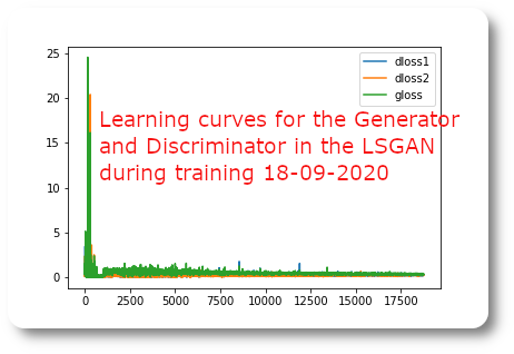
• I ran the SGAN example on my iMac. It took about 3 hours and 18 minutes. It seems to me that the quality of the images delivered with the SGAN are superior to the quality of the images provided by a LSGAN (Least Squares GAN):

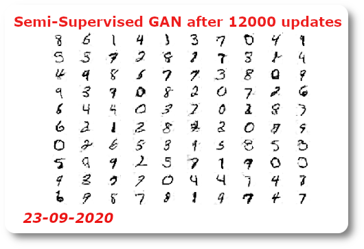
Handwritten digits generated with a Semi-Supervised GAN

• The quality of the generated images is good even the relatively small numbers of trains epochs.
• Then I evaluated the model using the entire training and test dataset with the different trained model obtained during the 10 epochs. The best performance was reached after 6600 batches:
• Train accuracy: 95.317%
• Test accuracy: 95.490%

PART VI: Image Translation

Chapter 21: Introduction to Pix2Pix

• Image-to-image translation is the controlled conversion of a given source image to a target image. An example might be the conversion of black and white photographs to color photographs. Image-to-image translation is a challenging problem and often requires specialized models and loss functions for a given translation task or dataset. The Pix2Pix GAN is a general approach for image-to-image translation. Pix2Pix GAN changes the loss function so that the generated image is both plausible in the content of the target domain, and is a plausible translation of the input image.
• "In analogy to automatic language translation, we define image-to-image translation, we define automatic image-to-image translation as the task of translating one possible representation of a scene into another, given sufficient training data." Image-to-Image Translation with Conditional Adversarial Networks, 2016.
• Pix2Pix is a Generative Adversarial Network, or GAN, model designed for general purpose image-to-image translation.
• Pix2Pix GAN is an implementation of the cGAN where the generation of an image is conditional on a given image.
• Both the generator and discriminator models use standard Convolution-BatchNormalization-Relu (Rectified Linear Activation Unit) blocks of layers as is common for deep convolutional neural networks.
• The generator model takes an image as input, and unlike a standard GAN model, it does not take point from the latent space as input. Instead, the source of randomness comes from the use of dropout layers that are used both during training and when a prediction is made.
• The Pix2Pix model uses a PatchGAN. This is a deep convolutional network designed to classify patches of an input image as real or fake, rather than the entire image.
• The generator model is trained using both the adversarial loss for the discriminator model and the L1 or mean absolute pixel difference between the generated translation of the source image and the expected target image.

Chapter 22: How to Implement Pix2Pix Models

• The Pix2Pix GAN is a generator model for performing image-to-image translation trained on paired examples. For example, the model can be used to translate images of daytime to nighttime, or from sketches of products like shoes to photographs of products. The benefit of the Pix2Pix model is that compared to other GANs for conditional image generation, it is relatively simple and capable of generating large high-quality images across a variety of image translation task.
• The Pix2Pix GAN has been demonstrated on a range of image-to-image translation tasks such as converting maps to satellite photographs, black and white photographs to color, and sketches of products to product photographs.
• « we design a discriminator architecture - which we term a PatchGAN - that only penalizes structure at the scale of patches. This discriminator tries to classify if each N × N patch in an image is real or fake. We run this discriminator convolutionally across the image, averaging all responses to provide the ultimate output of D »  Image-to-Image translation with Conditional Adversarial Networks, 2016
• Indeed, since the release of the pix2pix software associated with this paper, a large number of internet users (many of them artists) have posted their own experiments with our system, further demonstrating its wide applicability and ease of adoption without the need for parameter tweaking. 
• The PatchGAN configuration is defined using a shorthand notation as: C64-C128-C256C512, where C refers to a block of Convolution-BatchNorm-LeakyReLU layers and the number indicates the number of filters.
• Unlike traditional generator models in the GAN architecture, the U-Net generator does not take a point from the latent space as input. Instead, dropout layers are used as a source of randomness both during training and when the model is used to make a prediction, e.g. generate an image at inference time. Similarly, batch normalization is used in the same way during training and inference, meaning that statistics are calculated for each batch and not fixed at the end of the training process.
• Tanh activation function is used in the output layer, common to GAN generator models.
• The discriminator model can be updated directly, whereas the generator model must be updated via the discriminator model.

Chapter 23: How to Develop a Pix2Pix End-to-End

• The Pix2Pix Generative Adversarial Network, or GAN, is an approach to training a deep convolution always neural network for image-to-image translation tasks.The careful configuration of architecture as a type of image-conditional GAN allows for both the generation of large images compared to prior GAN models (e.g. such as 256 x 256 pixels) and the capability of performing well on a variety of different image-to-image translation tasks.
• The code provided in the book is developing the Pix2Pix model for translating satellite photos to Google maps images. The second part of the chapter is a piece of code that does the reverse: developing a Pix2Pix model to translate Google Maps to plausible image satellite.
• Other examples of Image-to-Image are provided.

Chapter 24: Introduction to the Cycle GAN

• Image-to-image translation involves generating a new synthetic version of a given image with a specific modification, such as translating a summer landscape to winter. Training a model for image-to-image translation typically requires a large dataset of paired examples. These datasets can be difficult and expensive to prepare, and in some cases impossible, such as photographs of paintings by long dead artists. The CycleGAN is a technique that involves the automatic training of image-to-image translation models without paired examples. The models are trained in an unsupervised manner using a collection of images from the source and target domain that do not need to be related in any way.
• The GAN architecture is an approach to training a model for image synthesis that is comprised of two models: a generator model and a discriminator model. The generator takes a point from a latent space as input and generates new plausible images from the domain, and the discriminator takes an image as input and predicts whether it is real (from a dataset) or fake (generated). Both models are trained in a game, such that the generator is updated to better fool the discriminator and the discriminator is updated to better detect generated images. The CycleGAN is an extension of the GAN architecture that involves the simultaneous training of two generator models and two discriminator models.
• The CycleGAN uses an additional extension to the architecture called cycle consistency. This is the idea that an image output by the first generator could be used as input to the second generator and the output of the second generator should match the original image. The reverse is also true: that an output from the second generator can be fed as input to the first generator and the result should match the input to the second generator. Cycle consistency is a concept from machine translation where a phrase translated from English to French should translate from French back to English and be identical to the original phrase. The reverse process should also be true.
• An excellent paper is describing all the possibilities of image translation with paintings of Monnet.

Part VII: Advanced GAN

Chapter 27: Introduction to the BIGGAN

• More recently, work has focused on the effective application of the GAN for generating both high-quality and larger images.
• BigGAN is designed for class-conditional image generation. That is, the generation of images using both a point from latent space and image class information as input.
• The contribution of the BigGAN model is the design decisions for both the models and the training process.

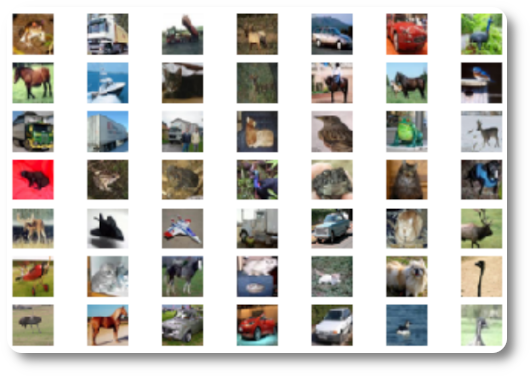
Set of images generated by a BIG GAN

Chapter 28: Introduction to the progressive Growing GAN

• Progressive growing GAN models are capable of generating photorealistic synthetic faces and objects at high resolution that are remarkably realistic.
• A problem with GANs is that they are limited to small dataset sizes, often a few hundred pixels and often less than 100-pixel square images.
• Generating high-resolution images is believed to be challenging for GAN models as the generator must learn how to output both large structure and fine details at the same time.
• Large images, such as 1024-pixel square images, also require significantly more memory, which is in relatively limited supply on modern GPU hardware compared to main memory.
• A solution to the problem of training stable GAN models for larger images is to progressively increase the number of layers during the training process.
• Progressive Growing GAN requires that the capacity of both the generator and discriminator model be expanded by adding layers during the training process.
• Unlike greedy layer-wise pre-training, progressive growing GAN involves adding blocks of layers and phasing in the addition of the blocks of layers rather than adding them directly.
• All existing layers in both networks remain trainable throughout the training process.
• 
  
  
  Examples of Photorealistic Generated Faces Using Progressive Growing GAN
  From Progressive Growing of GANs for Improved Quality, Stability and Variation

Chapter 29: Introduction to the StyleGAN

• The StyleGAN is an extension of the progressive growing GAN.
• The StyleGAN generator no longer takes a point from the latent space as input; instead, there are two new sources of randomness used to generate a synthetic image: a standalone mapping network and noise layers.
• The use of different style vectors at different points of the synthesis network gives control over the styles of the resulting image at different levels of detail. For example, blocks of layers in the synthesis network at lower resolutions (e.g. 4 × 4 and 8 × 8) control high-level styles such as pose and hairstyle. Blocks of layers in the middle of the network (e.g. as 16 × 16 and 32 × 32) control hairstyles and facial expression. Finally, blocks of layers closer to the output end of the network (e.g. 64 × 64 to 1024 × 1024) control color schemes and very fine details.
• A Style-Based Generator Architecture for Generative Adversarial Networks, 2018.
• A video explaining the capacity explained in the paper above is demonstrating a Style GAN generated images: very impressive.
• The code is free, so that you can apply it to your own set of images.
• 
  
  
  These  people are not real, they were produced by our generator that allows control over different aspects of the image
  
  

Conclusion

• This ends up the series of book from Jason Brownlee. 
• This book related to GAN is certainly the most complex but also the most interesting one as GAN are very promising.
• Big thanks to Jason Brownlee who leads me to this journey of deep neural network up to the most sophisticated neural network like the GANs.
• This post is only a summary of the book, the essence is in the book itself.

Generative Adversarial Network with Python (Part III and Part IV) Jason Brownlee

Preamble

•  This is a followup of previous post about the excellent book from Jason Brownlee: "Generative Adversarial Networks with Python"
• 
  
  
  
  
  Cercié en Beaujolais - Août 2020
  
  

Part III: GAN Evaluation

Chapter 11: How to Evaluate Generative Adversarial Networks

• Both the generator and discriminator are trained together to maintain an equilibrium.
• Models must be evaluated using the quality of the generated synthetic images.
• One training epoch refers to one cycle through the images in the training dataset used to update the model.
• Crowdsourcing platform like Amazon's Mechanical Turk.
• Two widely adopted metrics for evaluating generated images are the Inception Score and the Frechet Inception Distance. Like the inception score, the FID score uses the inception v3 model. The Frechet distance is also called the Wasserstein-2 distance. A lower FID score indicates more realistic images that match the statistical properties of real images.
• Once your confidence in developing GAN models improves, both the Inception Score and the Frechet Inception Distance can be used to qualitatively summarize the quality of generated images.

Chapter 12: How to Implement the Inception Score

• The Inception Score, or IS for short, is an objective metric for evaluating the quality of generated images, specifically synthetic images output by generative adversarial network models. 
• The score seeks to capture two properties of a collection of generated images: image quality and image diversity.

Chapter 13: How to Implement the Frechet Inception Distance

• The Frechet Inception Distance, or FID for short, is a metric that calculates the distance between feature vectors calculated for real and generated images.
• The difference of two Gaussians (synthetic and real-world images) is measured by the Frechet distance also known as Wasserstein-2 distance.

Part IV: GAN Loss

Chapter 14: How to Use Different GAN Loss Functions

• The GAN architecture is relatively straightforward, although one aspect that remains challenging for beginners is the topic of GAN loss functions. The main reason is that the architecture involves the simultaneous training of two models: the generator and the discriminator. The discriminator model is updated like any other deep learning neural network, although the generator uses the discriminator as the loss function, meaning that the loss function for the generator is implicit and learned during training.
• The generative adversarial network, or GAN for short, is a deep learning architecture for training a generative model for image synthesis. They have proven very effective, achieving impressive results in generating photorealistic faces, scenes and more.
• The generator is not trained directly and instead is trained via the discriminator model. Specifically, the discriminator is learned to provide the loss function for the generator.
• The choice of a loss function is a hot research topic and many alternate loss functions have been proposed and evaluated. Two popular alternate loss functions used in many GAN implementations are the least squares loss and the Wasserstein loss.
• Despite a very rich research activity leading to numerous interesting GAN algorithms, it is still very hard to assess which algorithm(s) perform better than others.

Chapter 15: How to Develop a Least Squares GAN (LSGAN)

• The generator is updated in such a way that it is encouraged to generate images that are more likely to fool the discriminator. The discriminator is a binary classifier and is trained using binary cross-entropy loss function.
• The choice of cross-entropy loss means that points generated far from the boundary are right or wrong, but provide very little gradient information to the generator on how to generate better images. This small gradient for generated images far from the decision boundary is referred to as a vanishing gradient problem or a loss saturation. The loss function is unable to give a strong signal as to how to best update the model.
• The LSGAN is a modification to the GAN architecture that changes the loss function for the discriminator from binary cross-entropy to a least squares loss. The motivation for this change is that the least squares loss penalize generated images based on their distance from the decision boundary. This will provide a strong gradient signal for generated images that are very different or far from the existing data and address the problem of saturated loss.
• The LSGAN can be implemented by using the target values of 1.0 for real and 0.0 for fake images and optimizing the model using the mean squared error (MSE) loss function, e.g. L2 loss. The output layer of the discriminator model must be a linear active function.
• The generator model is updated via the discriminator model. This is achieved by creating a composite model that stacks the generator on top of the discriminator so that error signals can flow back through the discriminator to the generator. The weights of the discriminator are marked as not trainable when used in the composite model.
• The LSGAN addresses vanishing gradients and loss saturation of the deep convolutional GAN.
• The LSGAN can be implemented by a mean squared error or L2 loss function for the discriminator model.
• I ran the code provided by Jason on my Anaconda configuration and iMac Hardware. The code is an example of training on a MNIST dataset.The training lasted 3 hours and 26 minutes on my iMac.

100 LSGAN Generated Handwritten Digits after 1 training epoch

100 LSGAN Generated Handwritten Digits after 20 training epochs

Learning curves for the Generator and Discriminator 

• I ran the code to infer a new set of handwritten digits by using the trained model saved previously for 20 epochs:

100 LSGAN generated plausible handwritten digits

• Once the model has been trained, the inference is very fast to generate and the numbers are quite plausible.

Chapter 16: How to Develop a Wasserstein GAN (WGAN)

• The Wasserstein Generative Adversarial Network, or Wasserstein GAN, is an extension to the generative adversarial network that both improves the stability when training the model and provides a loss function that correlates with the quality of generated images. The development of the WGAN has a dense mathematical motivation, although in practice requires only a few minor modifications to the established  deep convolutional generative adversarial network, or DCGAN.
• Instead of using a discriminator to classify or predict the probability of generated images as being real or fake, the WGAN changes or replaces the discriminator model with a critic that scores the realness or fakeness of a given image. This change is motivated by a mathematical argument that training the generator should seek a minimization of the distance between the distribution of the data observed in the training dataset and the distribution observed in generated examples. The argument contrasts different distribution distance measures, such as Kullback-Leibler (KL) divergence, Jensen-Shannon (JS) divergence, and the Earth-Mover (EM) distance, the latter also referred to as Wasserstein distance.
• The benefit of the WGAN is that the training process is more stable and less sensitive to model architecture and choice of hyper parameter configurations.
• The lower the loss of the critic when evaluating generated images, the higher the expected quality of generated images. This is important as unlike other GANs that seek stability in terms of finding an equilibrium between two models, the WGNA seeks convergence, lowering generator loss.
• The calculations are straightforward to interpret once we recall that stochastic gradient descent seeks to minimize loss.
• I ran the WGAN code provided in the book with the MNIST dataset, which consists at generating the number "7". The result I got was interesting, as we see that the network diverges around epoch #400 and then stabilizes again around epoch #800. The generated images are of better quality even after 194 batches compared to the images generated at batch # 776.

Loss and accuracy for a Wasserstein GAN (10 epochs)

• The images of the "7" generated at batch #194:
  
  The images generated at batch # 194
  
  

The images generated at batch # 776

The images generated at batch # 970

• I ran again the WGAN, this time the critics of the fake skyrockets after batch #600:

Loss and accuracy of a Wasserstein GAN (2nd trial, 10 epochs))

• So I decided to run with doubling the number of epochs:

Wasserstein GAN (3rd trial, 20 epochs)

• I had difficulty to interpret the learning curves with this WGAN. The only thing I am sure is the quality of the generated images: you can observe that at batch #776 the quality of the images are disastrous, whereas at batch # 970 they are quite better. The analysis from Jason Brownlee is the following: "WGAN is quite different from the typical GAN (DCGAN). The difference in loss means we cannot  interpret learning curves easily - if at all. For myself, I don't even try and instead try to focus on the images generated by the model".

• I ran the code to infer a new set of handwritten digit "7" by using the trained model saved previously for 20 epochs:

Sample of Generated Images of a Handwritten Number 7 at Epoch 1940 from a Wasserstein GAN

Conclusion

• The part IV of the book, GAN loss, was the most interesting. I have experimented the stochastic nature of a GAN.
• I will jump hastily into the next part of the book, part V: conditional GANs.
• Great thanks to Jason Brownlee, thanks to him I have enjoyed so much getting a new knowledge and at the same time practicing and experimenting GANs. 

Generative Adversarial Networks with Python (Part I and Part II) - Jason Brownlee

 

Introduction

• GANs are very promising and it is the reason why I bought this book of Jason Brownlee.
• It's the seventh book of Jason Brownlee that I am reading and practicing. 
• The way Jason Brownlee explains the concepts and the fact that code examples are provided are key elements for buying such books.
• In the book you will find the concepts explained from different point of view in in different chapters, or rephrased so that in the end you have a good chance to remember all these concepts.

Part 1: Foundations

Chapter 1: What are Generative Adversarial Networks

• Generative modeling is an unsupervised learning task in machine learning that involves automatically discovering and learning the regularities of patterns in input data in such a way that the model can be used to generate or output new examples that plausibly could have been drawn from the original dataset.
• GANs are a clever way of training a generative model by framing the problem as a supervised learning problem with two sub-models: the generator model that we train to generate new examples, and the discriminator model that tries to classify examples as either real (from the domain) or fake (generated). The two models are trained together in an adversarial zero-sum game until the discriminator model is fooled about half of the time, meaning the generator model is generating plausible examples.
• GANs are exiting in image-to-image translation tasks such as translating photos of summer to winter or day or night, and in generating photorealistic photos of objects, scenes, and people that even humans cannot tell are fake. Example below is impressive: 

Example of Progression in the capability of GAN. From the Malicious use of AI.

• Supervised: because there is a real expected outcome to which a prediction is compared. Examples of supervised learning problems include classification and regression, and examples of supervised learning algorithms include logistic regression and random forests.
• The second main type of machine learning is the descriptive or unsupervised learning approach. Here we are only given inputs, and the goal is to find "interesting patterns" in the data. This is a much less well-defined problem, since we are not told what kind of patterns to look for, and there is no obvious error metric to use (unlike supervised learning, where we can compare our prediction of y for a given x to the observed value). 

Page 2, Machine Learning: A Probabilistic Perspective, 2012.

• Examples of unsupervised learning algorithms are K-means and Generative Adversarial Networks.
• Classification is also traditionally referred to as discriminative modeling.
• Alternately, unsupervised models that summarize the distribution of input variables may be able to be used to create or generate new examples in the input distribution. As such, these types of models are referred to as generative models.
• In fact, a really good generative model may be able to generate new examples that are not just plausible, but indistinguishable from real examples from the problem domain.
• Examples of generative models: 
• Naive Bayes
• Latent Dirichlet Allocation (LDA)
• Gaussian Mixture Model (GMM)
• Restricted Boltzmann Machine (RBM)
• Deep Belief network (DBN)
• Variational Autoencoder (VAE)
• Generative Adversarial Network (GAN)
• The GAN model architecture involves two sub-models: a generator model for generating new examples and a discriminator model for classifying whether generated examples are real (from the domain) or fake (generated by the generator model).
• The two models, the generator and discriminator, are trained together.
• Successful generative modeling provides an alternative and potentially more domain-specific approach for data augmentation. In fact, data augmentation is a simplified version of generative modeling, although it is rarely described this way.

Chapter 2: How to Develop Deep Learning Models With Keras

• Activation functions that transform a summed signal from each neuron in a layer can be added to the Sequential as a layer-like object called the Activation class.
• The most common optimization algorithm is stochastic gradient descent, or sgd.
• Once the network is compiled, it can be fit, which means adapting the model weights in response to a train dataset. 
• The network is trained using the back propagation algorithm and optimized according to the optimization algorithm and loss function specified when compiling the model.
• Once fit, a history object is returned that provides a summary of the performance of the model during training. This includes both the loss and any additional metrics specified when compiling the model, recorded each epoch.
• Keras functional. models:
• The sequential API: allows you to to create models layer-by-layer for most problems. It is limited in that it does not allow you to create models that share layers or have multiple input or output layers.
• The functional API: is an alternate way of creating models that offers a lot more flexibility, including creating more complex models.
• When input data is one-dimensional (rows of samples), such as Mulitlayer Perceptron, the shape must explicitly leave room for the shape of the mini batch size used when splitting the data when training the network. Therefore the shape tuple is always defined with a hanging last dimension (2,).

Chapter 3: How to Upsample with Convolutional Neural Networks

• The generator model is typically implemented using a deep convolutional neural network and results-specialized layers that learn to fill in the features in an image rather than extract features from an image.
• Two common types of layers can be used in the generator model: upsample layer that simply doubles the dimensions of the input and the transpose convolutional layer that performs an inverse convolution operation.

upsampling

transposing

• The transpose convolutional layer is more complex than a simple upsampling layer. A simple way to think about it is that it both performs the upsample operation and interprets the coarse input data to fill in the detail while it is upsampling. It is like a layer that combines the UpSampling2D and Conv2D layers into one layer.
• In fact the transpose convolutional layer performs an inverse convolution operation. Specifically, the forward and backward passes of the convolutional layer are reversed.
• A deconvnet can be thought of as convnet model that uses the same components (filtering, pooling) but in reverse, so instead of mapping pixels to features does the opposite.
• GAN performance and skill is notoriously difficult to quantify.

Chapter 4: How to implement the GAN Training Algorithm

• Latent variable are variables that are not directly observed but are rather inferred from other variables that are observed.
• An epoch is defined as one cycle through a training dataset, where the samples in a training dataset are used to update the model weights in mini batch.
• The discriminator model must make predictions for the real and fake samples and the weights the discriminator must be updated proportional to how correct or incorrect those predictions were.
• Next, the generator model must be updated. Again, a batch of random points from the latent space must be selected and passed to the generator to generate fake images, and then passed to the discriminator to classify.
• The discriminator is trained to correctly classify real and fake images.
• "This is just the standard cross-entropy cost that is minimized when training a standard binary classifier with a sigmoid output. The only difference is that the classifier is trained on two minibatches of data; one coming from the dataset, where the label is 1 for all examples, and one coming from the generator, where the label is 0 for all examples." NIPS 2016 Tutorial: Generative Adversarial Networks, 2016

Chapter 5: How to Implement GAN Hacks to Train Stable Models

• There are a number of heuristics or best practices called GAN hacks that can be used when configuring and training your GAN models. These heuristics have been hard won by practitioners testing and evaluating hundreds or thousands of combinations of configuration operations on a range of problems over many years.
• GANs are difficult to train. The reason they are difficult to train is that both the generator model and the discriminator model are trained simultaneously in a game. This means that improvements to one model come at the expense of the other model. The goal of training two models involves finding a point of equilibrium between the two competing concerns.

Generator Model Architecture for the DCGAN

• Best practices for Deep Convolutional GANs (DCGANs):
• Downsample using Strided convolutions
• Upsample using strided convolution
• Use Leaky ReLU:
• The Rectified linear activation unit, or ReLU for short, is a simple calculation that returns the value provided as input directly, or the value 0.0 if the input is 0.0 or less. It has become a best practice when developing deep Convolutional Neural Networks generally.
• Use batch normalization:
• Batch Normalization standardizes the activations from a prior layer to have a zero mean and unit variance. This has the effect of stabilizing the training process. Batch normalization is used after the activation of convolution and transpose convolutional layers in the discriminator and generator models respectively.
• Use Gaussian weight initialization
• Before a neural network can be trained, the model weights (parameters) must be initialized to small random variables. The best practice for DCGAN models reported is to initialize all weights using a zero-centered Gaussian distribution (the normal or bell-shaped distribution) with a standard deviation of 0.02.
• Use Adam Stochastic Gradient Descent:
• Stochastic gradient descent, or SGD for short, is the standard algorithm used to optimize the weights of convolutional neural network models.
• Scale images to the range [-1, 1]:
• It is recommended to use the hyperbolic tangent activation function as the output from the generator model. As such, it is also recommended that real images used to train the discriminator are scaled so that their pixel values are in the range [-1, 1]. This is so that the discriminator well always receive images as input, real and fake, that have pixel values in the same range.
• Use a Gaussian latent space:
• The latent space defines the shape and distribution of the input to the generator model used to generate new images. The DCGAN recommends sampling from a uniform distribution, meaning that the shape of the latent space is an hypercube. The more recent best practice is to sample from a standard Gaussian distribution, meaning that the shape of the latent space is a hypersphere, with a mean of zero and a standard deviation of one.
• Separate batches of real and fake images:
• The discriminator model is trained using stochastic gradient descent with mini-batches. The best practice is to update the discriminator with separate batches of real and fake images rather than combining real and fake images into a single batch.
• Use label smoothing:
• It is common to use the class label 1 to represent real images and class label 0 to represent fake images when training the discriminator model. These are called hard labels, as the label values are precise or crisp. It is a good practice to use soft labels, such as values slightly more or less than 1.0 or slightly more than 0.0 for real and fake images respectively, where the variation for each image is random. This is often referred to as label smoothing and can have a regularizing effect when training the model.
• Use noisy labels:
• The labels used when training the discriminator are always correct. This means that fake images are always labeled with class 0 and real images are always labeled with class 1. It is recommended to introduce some errors to these labels where some fake images are marked as real, and some real images are marked as false.
• Soumith Chintals's GAN hacks

Part II: GAN Basics

Chapter 6: How to Develop a 1D GAN from Scratch

• A generator model is capable of generating new artificial samples that plausibly could have come from an existing distribution of samples.
• Importantly, the performance of the discriminator model is used to update both the model weights of the discriminator itself and the generator model.
• The weights in the generator model are updated based on the performance of the discriminator model. When the discriminator model is good at defecting fake samples, the generator is updated more (via a larger error gradient), and when the discriminator model is relatively poor or confused when detecting fake samples, the generated model is updated less. This defines the zero-sum or adversarial relationship between those two models.
• The back propagation process used to update the model weights will see this as a large error and will update the model weights (i.e. only the weights in the generator) to correct for this error, in turn making the generator better at generating plausible fake samples.
• The weights in the discriminator are marked as not trainable.

My first GAN

1D GAN: blue dots are generated one

Chapter 7: How to Develop a DCGAN for Grayscale Handwritten Digits

MNIST handwritten digit dataset extract

• The discriminator: 
• the model is trained to minimize the binary cross-entropy loss function, appropriate for binary classification. We will use some best practices in defining the discriminator model, such as the use of LeakyReLU instead of ReLU, using Dropout, and using the Adam version of stochastic gradient descent with a learning rate of 0.0002 and a momentum of 0.5.
• is just a normal neural network model for binary classification
• needs to be trained, this involves repeatedly retrieving samples of real images and samples of generated images and updating the model for a fixed number of iterations.
• The generator:
• we want many parallel versions or interpretations of the input. This is a pattern in convolutional neural networks where we have many parallel filters resulting in multiple parallel activation maps, called feature maps, with different interpretation of the input.
• the next major architectural innovation involves upsampling the low-resolution image to a higher resolution version of the image.
• is not compiled and does not specify a loss function or optimization algorithm. This is because the generator is not trained directly.
• Training the GAN model:
• a new GAN model can be defined that stacks the generator and discriminator such that the generator receives as input random points in the latent space and generates samples that are fed into the discriminator model directly, classified, and the output of this larger model can be used to update the model weights of the generator.
• therefore, we will mark all of the layers in the discriminator as not trainable when it is part of the GAN model so that they cannot be updated and overtrained on fake examples.
• therefore when the generator is trained as part of the GAN model, we will mark the generated samples as real (class = 1)
• making the discriminator not trainable is a clever trick in the Keras API. 

MNIST number generation after 100 epochs

performed on iMac during nearly 24 hours of training

• Comment of the above image: When viewing the discriminator model's accuracy in concert with generated images, we can see that the accuracy on fake examples (98%) does not correlate well with the subjective quality of the image, but the accuracy for real examples (15%) may. It is crude and possibly unreliable metric of GAN performance, along with loss.
• Then the code example provided in the book is a piece of code that generates 25 handwritten images:

25 GAN Generated MNIST handwritten images

• I observe that most of the images are plausible.
• There is also a piece of code that can produce a single digit, also very plausible:

a GAN Generated MNIST handwritten

Chapter 8: How to Develop a DCGAN for Small Color Photographs

• Developing a GAN for generating images requires both a discriminator convolutional neural network model for classifying wether a given image is real or generated and a generator model that uses inverse convolutional layers to transform an input to full two-dimensional image of pixel values.
• CIFAR is an acronym that stands for the Canadian Institute For Advanced Research. The dataset is comprised of 60 000 32x32 pixel color photographs of objects from 10 classes, such as frogs, birds, cats, ships, airplanes, etc...

Plot of the first 49 small objects from CIFAR-10

• The discriminator model has no pooling layers and a single node in the output layer with the sigmoid activation to predict whether the input sample is real or fake. The model is trained to minimize the binary cross-entropy loss function, appropriate for binary classification.
• It helps to see that the discriminator is just a normal neural network model for binary classification.
• The generator model will generate images with pixel values in the range [-1, 1] as it will use Tanh activation function, a best practice.
• We don't want just one low-resolution version of the image; we want many parallels versions or interpretations of the input. This is a pattern in Convolutional Neural Networks where we have many parallel filters resulting in multiple parallel activation maps, called feature maps, with different interpretations of the input.
• The generator model is not compiled and does not specify a loss function or optimization algorithm.

CIFAR-10 generated untrained

100 CIFAR images generated by a GAN

GAN Generated CIFAR model for a Specific Point in the latent space

Chapter 9: How to Explore the Latent Space When Generating Faces

• The generative model in the GAN architecture learns to map points in the latent space to generated images.
• "Unsupervised Representation Learning with Deep Convolutional Generative Adversarial Networks": the authors explored the latent space for GANs fit on a number of different training datasets, most notably a dataset of celebrity faces. They demonstrated two interesting aspects:
• The first was the vector arithmetic with faces. For example, a face of a smiling woman minus the face of a neutral woman plus the face of a neutral man resulted in the face of a smiling man:
• smiling woman - neutral woman + neutral man = smiling man
• The second demonstration was the transition between two generated faces, specifically by creating a linear path through the latent dimension between the points that generated two faces and the generating all of the faces for the points along the path.
• When working with a GAN, it is easier to model a dataset if all of the images are small and square in shape. 
• The pre-trained Multi-Task Cascaded Convolutional Neural Network (MTCNN) is used.
• We need inputs for the generator model: these are random points from the latent space, specifically Gaussian distributed random variables.
• In these cases, we have performed a linear interpolation which assumes that the latent space is a uniformly distributed hypercube. Technically, our chosen latent space is a 100-dimension hypersphere or multimodal Gaussian distribution. There is a mathematical function called the Spherical linear interpolation function, or Slerp, that should be used when interpolating this space to ensure the curvature of the space is taken in to account.
• Sadly my GAN example ran in collapse mode at epoch #6 after 10 hours of running on my iMac:
• 
  
  
  GAN collapsed on iMac after 10 hours

• The AWS p3 EC2 instance being not part of the free Amazon offer, I decided not to run the image face generation example on AWS. May be later.

Chapter 10: How to Identify and Diagnose GAN Failure modes

• GANs are difficult to train. The reason they are difficult to train is that both the generator model and the discriminator model are trained simultaneously in a zero sum game. This means that improvements to one model come at the expense of the other model.
• The discriminator model is trained separately, and as such, the model weights are marked as not trainable in this larger GAN model to ensure that only the weights of the generator model are updated.
• Stable GAN:
• Discriminator loss on real and fake images is expected to sit around 0.5
• Generator loss on fake images is expected to sit between 0.5 and perhaps 2.0
• Discriminator accuracy on real and fake images is expected to sit around 80%
• Variance of generator and discriminator loss is expected to remain modest
• The generator is expected to produce its highest quality image during a period of stability
• Training stability may degenerate into periods of high-variance loss and corresponding lower quality generated images.
• There are two failures cases that are common to see when training GAN models on new problems; they are mode collapse and convergence failure.
• I cannot reach the results indicated in the book about the stable GAN and the collapsed GAN. Very rapidly, after 19 iterations, the discriminator reaches 100% on real and 100% on fake:
• >19, d1=0.059, d2=0.093 g=0.315, a1=100, a2=100
• Analysis after 250 iterations: >260, d1=0.001, d2=0.001 g=0.001, a1=100, a2=100
• The loss of the discriminator decrease to a value close to zero.
• The loss for the generator decrease also to a value close to zero.
• The quality of the generated images are of very low quality:
  
  GAN Generated images are all the same in collapsed mode
  
  

These are the properties of a GAN convergence failure.

Line plots and accuracy for a Generative Adversarial Network with a convergence failure

Conclusion

• I am stopping here reading the first two parts of the book, FOUNDATIONS and GAN BASICS. GAN are complex and needs computing ressources such as for example Amazon Web Services EC2 with a Community AMI which is not part of the free AWS service offer. 
• I cannot run the GAN examples provided in the book on my iMac. AWS EC2 is mandatory to run GANs examples provided in the book, and the AWS free offer is not suitable. 
• The remaining parts of the book are:
• GAN Evaluation
• GAN Loss
• Conditional GANs
• Advanced GANs
• I will go through these four remaining parts once I have decided to hook up on a real GAN project.
• The GANs are very promising.
• Thanks to Jason Brownlee for providing such practical knowledge.