dimanche, décembre 13, 2020

Data Preparation for Machine Learning - Part I, II, III - Jason Brownlee

 Preamble


Chapter 4: Data Preparation Without Data Leakage

  • Naive application of data preparation methods to the whole dataset results in data leakage that causes incorrect estimates of model performance.
  • Data preparation must be prepared on the training set only in order to avoid data leakage.
  • Normalize data: scale input variables to the range 0-1
  • Standardization estimates the mean and standard deviation values from the domain in order to scale the variables.
  • The k-fold cross-validation procedure generally gives a more reliable estimate of model performance than a train-test split.

Part III: Data Cleaning

Chapter 5: Basic Data Cleaning

Chapter 6: Outlier Identification and Removal

  • Standard Deviation Method
    • 1 standard deviation from the mean covers 68% of data
    • 2 standard deviations from the mean covers 95 percent of data
    • 3 standard deviations from the mean covers 99,7% of data
  • Three standard deviations from the mean is a common cut-off in practice for identifying outliers in a Gaussian or Gaussian-like distribution.
  • Interquartile Range Method
    • Not all data is normal or normal enough to treat it as being drawn from a Gaussian distribution. A good statistic for summarizing a non-Gaussian distribution sample of data is the interquartile Range or IQR. The IQR is calculated as the difference between the 75th and 35th percentiles of the data and defines the box in a box and whisker plot.
    • We can calculate the percentiles of a dataset using the percentile() NumPy function.
  • Automatic Outlier Detection
    • Each example is assigned a scoring of how isolated or how likely it is to be outliers based on the size of its local neighborhood.
    • The scikit-learn library provides an implementation of this approach in the LocalOutlierFactor class.
  • Standard deviation and interquartile range are used to identify and remove outliers from a data sample.

Chapter 7: How to Mark and Remove Missing Data

  • Pandas provides the dropna() function that can be used to drop either columns or rows with missing data.

Chapter 8: How to Use Statistical Imputation

  • Datasets may have missing values, and this can cause problems fro many machine learning algorithms. As such, it is good practice to identify and replace missing values for each column in your input data prior to modeling your prediction task. This is called missing data imputation, or imputing for short. A popular approach for data imputation is to calculate a statistical value for each column (such as a mean) and replace all missing values for that column with the statistic.
  • Missing values must be marked with NaN values and can be replaced with statistical measures to calculate the column of values.
  • The scikit-learn machine learning library provides the SimpleImputer class that supports statistical imputation.
  • To correctly apply statistical missing data imputation and avoid data leakage, it is required that the statistics calculated for each column are calculated on the train dataset only, then applied to the train and test sets for each fold in the dataset. This can be achieved by creating a modeling pipeline where the first step is the statistical imputation, then the second step is the model. This can be achieved using the Pipeline class.
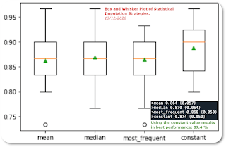
  • Testing different imputed strategies. The author proposes to test different strategies when replacing data by comparing the mean, the median, the mode (most frequent) and constant(0) strategies. 
Box and Whisper plot of different imputation strategies
  • We can see that the distribution of accuracy scores for the constant strategy may be better than the other strategies.

Chapter 9: How to Use KNN Imputation

  • Although any one among a range of different models can be used to predict the missing values, the k-nearest neighbor (KNN) algorithm has proven to be generally effective, often referred to as nearest neighbor imputation.
  • Missing values must be marked with NaN values and can be replaced with nearest neighbor estimated values.
  • An effective approach to data imputing is to use a model to predict the missing values.
  • One popular technique for imputation is a K-nearest neighbor model. A new sample is imputed by finding the samples in the training set "closest" to it and averages these nearby points to fill in the value.
  • The use of a KNN model to predict or fill missing values is referred to as Nearest Neighbor Imputation or KNN imputation.
  • The scikit-learn machine learning library provides the KNNImputer class that supports nearest neighbor imputation.
  • The KNNImputer is a data transform that is first configured based on the method used to estimate the missing values.

Chapter 10: How to Use Iterative Imputation

  • Missing values must be marked with NaN values and can be replaced with iteratively estimated values.
  • It is common to identify missing values in a dataset and replace them with a numeric value. This is called data imputing, or missing data imputation. One approach to imputing missing values is to use an iterative imputation model.
  • It is called iterative because the process is repeated multiple times, allowing ever improved estimates of missing values to be calculated as missing values across all features are estimated. This approach may be generally referred to as fully conditional specification (FCS) or multivariate imputation by chained equations (MICE).
  • Different regression algorithms can be used to estimate the missing values for each feature, although linear methods are often used for simplicity.
  • The scikit-learn machine learning library provides the IterativeImputer class that supports iterative imputation.

Conclusion

  • In this first three parts of the Data preparation for Machine Learning Book, we review the main data cleaning possibilities.
  • The following part will be related to "Feature Selection".

samedi, décembre 05, 2020

Comment décider - Annie Duke

Préambule

  • Ce post se veut un résumé des meilleurs extraits du livre de Annie Duke, "How to Decide".

Introduction

  • Un bon outil d'aide à la decision cherche à réduire le rôle des biais cognitifs. (tel que l'excès de confiance, le biais rétrospectif ou le biais de confirmation).
  • Une liste de "pour" et "contre" à tendance à amplifier le rôle des biais. 
  • Evaluer si une décision est bonne ou mauvaise revient à examiner les croyances qui ont informé la décision, les différentes options, et comment le futur pourrait se dérouler en fonction des choix.
  • Il faut éviter les pièges de la prise de décision en équipe, et spécialement la pensée de groupe.

Chapitre 1 : Le biais du résultat

  • Le biais de résultat (resulting bias) est un raccourci que l'on prend pour juger de la qualité d'une décision en fonction de la qualité du résultat.
  • L'expérience est supposée être notre meilleur professeur, mais parfois nous lions trop directement la qualité d'un résultat à la qualité de la décision.
  • Prendre de meilleures décisions signifie faire une meilleure prévision des différents scénarios.
  • On a tendance à remarquer lorsqu'on pas de chance et à oublier lorsque c'est un coup de bol.

  • Le biais de résultat fait que nous manquons de compassion pour nous-même et pour les autres.
  • On se flagelle lorsque les choses ne fonctionnent pas comme on l'aurait espéré.
  • La chance est ce qui intervient entre ta décision et le résultat. Le biais de résultat enlève la perception de la chance.
  • Quand tu prends une décision, tu peux rarement prédire un bon résultat. L'objectif est de choisir l'option qui va conduire à un ensemble de résultats potentiellement positif.
  • Tu prends une décision basée sur un nombre d'informations insuffisantes.

Chapitre 2 : Le biais rétrospectif

  • Afin d'évaluer la qualité d'une décision et d'en apprendre les leçons, tu as besoin d'évaluer ton état d'esprit honnêtement et te rappeler qu'est-ce que tu savais et qu'est-ce que tu ne savais pas avant la décision.
  • Les faits influent sur ta mémoire de ce que tu savais avant les faits.
  • Nous sommes généralement très prompts à critiquer celui qui a pris la décision, en négligeant de se mettre nous-mêmes dans la peau du décideur au moment de la décision.
  • Le biais rétrospectif ("hindsight bias") est la tendance à croire que le résultat était prévisible ou inéluctable.
  • Le biais rétrospectif, comme le biais du résultat, se manifeste par une influence trop importante du résultat. Le résultat vous empêche de voir ce que tu savais au moment de la décision.
  • L'extension dans votre mémoire ("memory creep") est le fait que les faits envahissent votre mémoire de ce que vous saviez avant la décision.

Chapitre 3 : La décision qui ouvre des univers multiple

  • La checklist décisionnelle t'aidera à qualifier la qualité de la décision en créant un arbre de décision. Pour cela il faut :
    1. Identifier la décision
    2. Identifier le résultat actuel
    3. Avec le résultat, créer un arbre avec les autres résultats qui étaient possibles au moment de la décision.
    4. Analyser les autres résultats afin de mieux comprendre qu'est-ce qu'il faut retenir du résultat actuel.
  • Le résultat seul ne te permet pas de dire si une décision était bonne ou mauvaise.
  • Il y a une asymétrie dans notre volonté de remettre les résultats dans leur contexte : on le fait plus facilement lorsqu'on échoue que lorsqu'on réussit.
  • Tu ne peux pas complètement apprendre d'un résultat sans comprendre les autres évènements qui auraient pu se produire.
  • Et si ? Un résultat possible d'une décision est un résultat qui ne sait pas produit. Une imagination.

Chapitre 4 : Préférences, bénéfices et probabilités

  • Six étapes pour une meilleure prise de décision
    1. Identifier le jeu des résultats, des issues possibles.
    2. Identifier vos préférences par association des bénéfices pour chaque résultat, issue ou objectif. Jusqu'à quel niveau de satisfaction vous appréciez le résultat en fonction de vos valeurs.
    3. Estimer la probabilité de chaque réalisation potentielle.
    4. Estimer la probabilité du résultat que vous aimez et que vous n'aimez pas pour l'option considérée.
    5. Répéter les étapes 1 à 4 pour les autres options.
    6. Comparer les options entre elles
  • Identifier l'ensemble des résultats possibles pour une prise de décision est déjà une amélioration énorme par rapport à une décision prise sur le résultat d'une décision passée.
  • La poubelle d'une personne est le trésor d'une autre personne.
  • Demander l'avis est un excellent outil décisionnel tant que tu es explicite sur tes objectifs et tes valeurs.
  • La taille du bénéfice est importante.
    • Si tu fais un investissement qui te rapporte de l'argent, c'est un gain. Si tu perds de l'argent, c'est une perte.
    • Le bénéfice peut être non monétaire : bonheur, temps, amélioration personnelle, estime de soi, santé, gentillesse
    • Evaluer la qualité d'une décision consiste à comprendre si les avantages sont valables par rapport aux risques des inconvénients.
  • Un des plus gros obstacles à une bonne prise de décision est de croire que la décision est bonne ou mauvaise et qu'il n'y a rien entre ces deux choix.
  • Une bonne prise de décision passe par la volonté de deviner.
  • Tu sais forcément quelque chose, et ce quelque chose est mieux que rien.
  • Qu'est-ce que je sais déjà et qui rendra mon estimation plus étayée ?
  • Qu'est-ce que je peux trouver qui m'aidera dans ma prise de décision ?
  • Ton choix est toujours une estimation des différents scénarios possibles.
  • Pour beaucoup de décisions, il y a souvent un aspect très particulier qui vous intéresse.
  • Ajouter des probabilités à un arbre décisionnel va améliorer de manière significative la qualité de vos décisions par rapport à simplement identifier les possibilités à vos préférences.
  • Si tu ne poses pas la question, tu n'auras pas la réponse.
  • Tu peux obtenir un certain contrôle sur l'incertitude qui se cache derrière l'imperfection de l'information.

Chapitre 5: Le pouvoir de la précision

  • Beaucoup de choses que tu ne connais pas se trouvent dans la tête d'autres personnes. Aussi obtenir du feedback des autres sur les choses que tu crois et les décisions que tu prends sera le meilleur outil pour extraire la connaissance du monde.
  • Pour avoir un feedback de qualité sur tes décisions et tes croyances, tu dois parler le même langage que la personne qui te donne le feedback.
  • Si tu crois qu'un évènement à 30% de chances de se passer et que tu parles avec quelqu'un qui a une information fiable que cet évènement se déroulera avec 70% de chances, cela te sera utile pour lever le désaccord.
  • La précision enlève le désaccord.
  • La précision est importante.
  • Qu'est-ce que je sais, et qu'est-ce que je peux apprendre ? 
  • Quand tu exprimes quelque chose avec certitude, les autres seront moins enclins à te contredire. Soit parce que ils pensent qu'ils ont torts et ne veulent pas s'embêter en partageant ce qu'ils pensent, ou ils pensent que tu as tort et ils ne veulent pas te mettre dans l'embarras. Ceci est un problème si tu as un rôle de leader.
  • Quand tu crées une limite inférieure et une limite supérieure, tu exprimes que tu te trouves quelque part entre pas de connaissance et une connaissance parfaite. Si tu laisses comprendre à celui qui t'écoute que tu n'est pas sûr fera que cette personne sera plus enclin à te partager de l'information utile parce que tu as demandé de l'aide.
  • Approche la qualité de ton information avec plus de scepticisme. Ce scepticisme te rendra plus curieux à questionner tes propres certitudes et plus enclin à chercher ce que les autres savent. Et ceci améliorera la qualité de tes décisions.
  • Fais en une habitude de te questionner toi même : si je me trompais, quelle serait l'alternative ?
  • Utilise la méthode du choc test pour savoir si tes limites inférieures et supérieures sont raisonnables.  Est-ce que tu serais vraiment choqué si la réponse correcte était en dehors des limites ?
  • Etre trop confiant en soi contrarie la prise de décision.

Chapitre 6 : prendre des décisions avec l'aide de l'extérieur

  • Ce que tu vois très clairement chez les autres est difficile de voir pour soi-même.
  • Votre perspective n'est pas si bonne quand tu es au centre.
  • Tes croyances créent un embouteillage pour la bonne prise de décision.
  • C'est très dur pour nous de voir le monde d'un point de vue extérieur.
  • Biais de confirmation : notre tendance à noter, interpréter et chercher de l'information qui confirme nos croyances.
  • Biais de non confirmation : notre tendance à appliquer plus d'importance à une information qui contredit nos croyances par rapport à une information qui confirme nos croyances.
  • Surconfiance : surestimation de nos compétences qui interfèrent avec notre capacité de prendre des décisions en se basant sur ces estimations.
  • Biais de fréquence : la tendance à sur estimer la fréquence de certains évènements  qu'il est facile de se rappeler parce qu'ils sont vivaces ou parce que nous les avons vécus plusieurs fois.
  • Biais du récent : croire que les évènements récents sont plus susceptibles de se reproduire qu'ils ne le sont réellement.
  • Biais de l'illusion du contrôle : surestimation de notre capacité à contrôler les évènements. En d'autres termes, sous-estimer l'influence de la chance.  
  • L'intérêt d'avoir le point de vue des autres est que même s' ils disposent des mêmes faits, ils peuvent voir les choses de manière différente.
  • Si tu veux te créer un outil d'aide à la décision qui amplifie les biais , cela devrait ressembler à une list de pour et de contre.
  • Si tu n'as pas une vue précise de tes compétences, tu peux prendre de très mauvaises décisions.
  • C'est inconfortable de penser à l'échec, mais cela vaut le coup de vivre dans cet inconfort parce que tu seras mieux préparé si les choses ne se passent pas comme dans ton idéal.
  • Les gens brillants sont meilleurs pour construire des arguments convaincants qui soutiennent leurs point de vue et qui renforcent les choses auxquelles ils croient.
  • La personne que tu as le plus de chance d'induire en erreur est toi-même. Et tu ne t'en rends pas compte parce que tu le vis de l'intérieur.
  • Remercie les gens qui, de bonne foi, sont en désaccord avec toi car c'est une action aimable de leur part.
  • Cherche le point de vue extérieur avec un esprit ouvert. 

Chapitre 7 : casser la paralysie de l'analyse ou comment optimiser le temps de votre prise de décision 

  • Le temps est une ressource limitée que tu dois dépenser avec sagesse.
  • La capacité de savoir quand il faut décider rapidement, ou quand il faut ralentir est une compétence cruciale à développer.
  • Tu dois être concentré sur les façons d'extraire les informations du monde afin de transformer l'univers de ce que tu ne connais pas dans quelque chose que tu connais.
  • Plus tu connais tes préférences, plus il te sera facile de prendre des décisions.
  • Le test du bonheur : demande toi si la décision que tu prends, bonne ou mauvaise, aura des chances significative sur ton bonheur dans un an. Si la réponse est non, la décision passe le test, ce qui signifie que tu peux prendre ta décision rapidement.
  • Les choix qui se répètent aident à diminuer le regret.
  • Lorsque le même type de décision revient couramment, tu as donc des chances répétées de faire ton choix, en y incluant même des choix que tu as rejeté dans le passé.
  • Freeroll : une situation dans laquelle il y a une asymétrie entre les avantages et les inconvénients car les pertes potentielles sont insignifiantes.
  • Le concept de freeroll est un modèle mental utile pour cibler des opportunités à saisir rapidement.
  • Plus tu t'engages rapidement et moins l'opportunité à des chances de disparaître.
  • L'impact de la décision obscurcit le freeroll.
  • La peur de l'échec ou du rejet peut vous paralyser.
  • Quelque soit l'option que je prends, quelle sera ma plus grande perte ?
  • Plus tu as un grand nombre d'options, plus il y a de chances qu'une de ces options te semble intéressante. Plus tu auras des options qui te semblent intéressantes, plus tu passeras ton temps dans la paralyse de l'analyse.
  • C'est le paradoxe : plus de choix signifie plus d'anxiété.
  • Pour toute décision, passe ton temps à départager les choses que tu aimes de celles que tu n'aimes pas.
  • Le coût de l'opportunité : quand tu choisis une option, tu perds le gain potentiel associé aux options que tu ne choisies pas.
  • Plus les gains associés aux options que tu ne choisies pas sont grands, plus le coût de l'opportunité est grand.
  • Si je prends cette option, qu'est-ce qu'il m'en coutera de l'abandonner ?

Chapitre 8 : la puissance de la pensée négative

  • Pensez positivement, mais planifiez négativement.
  • Ne confonds pas la destination avec la route.
  • Si cela devait mal se passer, de quelle manière cela se passerait-il ?
  • Lorsqu'il s'agit de navigation, la pensée négative vous permet d'arriver à destination de manière plus sûre.
  • Le contraste mental est le processus d'imagination des obstacles qui pourraient surgir sur la route de votre destination. 
  • La douleur mentale vous conduit aux gains réels.
  • Le biais du statu quo : la tendance à croire que les choses d'aujourd'hui seront les mêmes demain.
  • Analyse pré-mortem : tu t'imagines quelque part dans le futur après avoir échoué sur un objectif, et tu regardes derrière toi sur comment tu en es arrivé là.
  • Plus tu auras une vue large et complète sur ton futur, plus facile sera ta décision.
  • La valeur ajoutée de l'analyse pré-mortem pour les groupes : tu ajoutes plus de matière grise.
  • De manière intuitive, nous pensons que plusieurs cerveaux sont meilleurs qu'un seul pour la prise de décision.
  • Les analyses pré-mortem de groupe permettent d'exposer et encouragent les différents points de vue.
  • De même que la précision se trouve à l'intersection entre la vue externe et la vue interne, la vue la plus précise du futur se trouve à l'intersection entre l'analyse pré-mortem et le "backcasting".
  • La vue externe permet de discipliner les biais cognitifs qui résident dans la vue interne.
  • La table d'exploration de la décision.

  • La première chose que tu devrais considérer après un travail pré-mortem et un backcasting est de savoir si tu modifies ton objectif ou si tu changes de décision.
  • Rechercher les manières de mitiger l'impact des mauvaises surprises si elles arrivent.
  • De même qu'Ulysse, tu peux physiquement t'empêcher de prendre des mauvaises décisions.
  • Combien de fois j'ai fait exception à la règle récemment ?
  • Lors de l'occurence d'un mauvais résultat, il est difficile de voir la situation de façon rationnelle.
  • Vous compromettez la qualité de votre décision lorsque votre état émotionnel est intense suite à un mauvais résultat.
  • Est-ce que tu prends les choses de manière personnelle ? ou est-ce que tu entres dans la confrontation ? ou est-ce que tu utilises un langage particulier ? ou est-ce que tu t'engages dans des chemins de pensée lorsque tu es guidé par l'émotion ? Si oui alors tu es dans le mode "Tilt"

Chapitre 9 : l'hygiène de la décision. 

  • Le problème lorsque vous proposez d'abord votre opinion lorsque vous demandez un conseil à quelqu'un est que cela augmente de manière significative le fait qu'il exprimera la même opinion que vous. (Salomon Asch)
  • Un des meilleurs outils pour améliorer ta prise de décision est de demander le point de vue des autres. Mais tu ne peux le faire que si tu demandes leur vrai point de vue au lieu de voir votre perspective renvoyée.
  • Quand vient le moment de la décision, il est plus intéressant d'avoir plus de cerveaux qu'un seul. 
  • Si tu proposes d'abord ton avis, l'opinion de celui qui répond peut changer, ou la personne peut ne pas vouloir dire sa vraie pensée, ou elle peut penser qu'elle à tort.
  • Il est impossible de tomber dans le piège du biais rétrospectif si tu ne connais pas le résultat.
  • Si tu connais le résultat cela détruit le feedback.
  • Le fait que tu ne communiques pas le résultat et tes croyances avant de demander le feedback à une personne fait que cette personne se trouve dans les mêmes conditions que toi au moment de la décision.
  • Il faut solliciter le feedback de manière indépendante.
  • Eliciter le feedback de manière indépendante et partager le avec le groupe avant le meeting.
  • Il faut rendre anonyme le feedback.
  • L'effet de halo est un biais cognitif dans lequel une impression positive sur une personne dans un domaine vous fera aussi donner une une opinion positive de cette personne sur un problème tout autre.
  • La qualité de l'information que vous donnez avant la demande de feedback est très importante. Vous devrez préciser vos objectifs, ce qui pour vous à de la valeur et vos ressources.

samedi, novembre 14, 2020

Better Deep Learning - Jason Brownlee - Models Weights Ensembles

 Preamble

  • This blog post is an extract of the book "Better Deep Learning" from Jason Brownlee. 
  • This blog post is related to "Better Predictions": Combine Model Parameters with average Model Weights Ensemble(Chapter 26)

Chenonceaux

Chapter 26: Combine Model Parameters with Average Model Weights Ensemble

  • The model at the end of a training may not be stable or the best performing set of weights may not be usable as a final model. 
  • One approach to address this problem is to use an average of the weights from multiple models seen toward the end of the training run. This is called Polyak-Ruppert averaging and can be further improved by using a linearly or exponentially decreasing weighted average of the model weights. In addition to resulting in a more stable model, the performance of the averaged model weights can also result in better performance.
  • Learning the weights for a deep neural network model requires solving a high-dimensional non-convex optimization problem. A challenge with solving this optimization is that there are many good solutions and it is possible for the learning algorithm to bounce around and fail to settle in on one. In the area of stochastic optimization, this is referred to as problems with the convergence of the optimization algorithm on a solution, where a solution is defined by a set of specific weights values.
  • "Polyak averaging consists of averaging together several points in the trajectory through parameter space visited by an optimization algorithm."
  • "The basic idea is that the optimization algorithm may leap back and forth across a valley several times without ever visiting a point near of the bottom of the valley. The average of all the locations on either side should be close to the bottom of the valley though" - Deep Learning.
  • The simplest implementation of Polyak-Ruppert averaging involves calculating the average of the weights of the models over the last few trains epochs.
  • This can be improved by calculating a weighted average, where more weight is applied to more recent models, which is linearly decreased through prior epochs. An alternative and more widely approach used approach is to use an exponential decay in the weighted average.

Case Study

  • Multiclass Classification problem

Plot of a multi class classification samples

  • Multilayer Perceptron Model: in the problem suggested by the author, the training dataset is relatively small. There is a 10:1 ratio of examples in the training dataset to the holdout dataset. This mimics a situation where we may have a vast number of unlabeled examples and a small number of labeled examples with which to train a model. We will create 1100 data points. The problem will be trained for the first 100 points, 1000 will be held back in a test dataset, unavailable to the model.

Plot of Learning Curves of Accuracy on Train and Test Datasets

  • The preliminary step before working on a Model Weight Ensemble consists at saving model weights to file during training, and later combine the weights from the saved models in order to make a final model.
  • So, after this first step that establishes a baseline, the author suggest to create a new model from multiple existing models with the same architecture.
  • Each model has a get_weights() function that returns a list of arrays, one for each layer in the model.
  • After saving, loading and fitting with the weights the model, we are now ready to do some predictions.

Predictions with an Average Model Weight Ensemble


Plot of single Model test Performance and Model Weight Ensemble

Predictions with a Linear Weighted Average Ensemble


Accuracy of a linear Weighted Average Ensemble 
  • I notice that the linear weight weighted average ensemble is not better the average model weighted ensemble. This is not what I was expected. The results in fact vary given the stochastic nature of the learning algorithm.
Predictions with an Exponentially Decreasing Average Ensemble


Accuracy of Single And Ensemble Model Weight Ensemble with an Exponential Decay

Conclusion

  • Creating a model with the average of the weights from models observed towards the end of a training can result in a more stable and sometimes better-performing solution.
  • This was the last chapter of "Better Deep Learning" book from Jason Brownlee. 
  • I am very grateful to Jason Brownlee as this book helped me very much in my understanding of the tuning of neural networks.

vendredi, novembre 13, 2020

Better Deep Learning - Jason Brownlee - Stacked Generalization Ensemble

 Preamble

  • This blog post is an extract of the book "Better Deep Learning" from Jason Brownlee. 
  • This blog post is related to "Better Predictions": how to combine predictions with Stacked Generalization Ensembles (chapter 25)

Alpine A310

Chapter 25: Learn to combine Predictions with Stacked Generalization
  • Model averaging is an ensemble technique where multiple submodels contribute equally to a combined prediction. Model averaging can be improved by weighting the contributions of each submodel to the combined prediction by the expected performance of the submodel.This can be extended further by training an entirely new model to learn how to best combine the contributions from each submodel. This approach is called stacked generalization, or stacking for short, and can result in better predictive performance than any single contributing model.
  • Stacked generalization is an ensemble method where a new model learns how to best combine the predictions from multiple existing models.
  • Stacked generalization (or stacking) (Wolpert, 1992) is a different way of combining multiple models, that introduces the concept of a meta learner. Although an attractive idea, it is less widely used than bagging and boosting. Unlike bagging and boosting, stacking may be (and normally is) used to combine models of different types. The procedure is as follows:

    1. Split the training set into two disjoint sets.
    2. Train several base learners on the first part.
    3. Test the base learnerson the second part.
    4. Using the predictions from 3) as the inputs, and the correct responses as the outputs, train a higher level learner.
  • Note that steps 1) to 3) are the same as cross-validation, but instead of using a winner-takes-all approach, we combine the base learners, possibly nonlinearly.

Case Study

  • We are going to experiment the technique of "Stacked Generalization Ensembles" on a multi class classification problem. We will try to solve this classification problem with a classical MLP to establish a baseline, then in a second phase we will experiment the technique of Stacked Generalization Ensembles.

Plot of samples

  • Then we run our MLP on the samples. The author suggests to create a sample of 1100 data points, the model being trained only on the first 100 points and the remaining 1000 points are held back in a test dataset.

Learning curves of Model Accuracy on Train and Test Dataset

First experimentation: a separate stack model 

  • We start by training multiple submodels and saving them to files for later use in our stacking ensembles.
  • We then train a meta-learner that will best combine the predictions from the submodels and we will see if the performance is better.
    • The author prepare a training dataset for the meta-learner by providing examples from the test set to each of the submodels and collecting the predictions: dstack() and reshape() NumPy functions are used for combining arrays.
    • The meta-learner is trained with a simple logistic regression algorithm from the scikit-learn library. The LogisticRegression class supports multi class classification (more than two classes) using a multinomial scheme.  
  • Once fit the stacked model is used to make predictions on new data.

Fitting a logistic regression stacking model

  • From the image above, the result of the experimentation is that the stacked model with a performance of 83,4 % outperforms all single model accuracy.

Second experimentation: an integrated stack model

  • When using neural networks as submodels, it may be desirable to use a neural network as a meta-learner. Specifically, the sub-networks can be embedded in a larger multi-headed neural network that then learns how to best combine the predictions from each input submodel.
  • The graph of the stacked model:

Stacked Generalization Ensemble of Neural Network Models

  • The result of this stacked model is better that the separated one: 83,8% of accuracy compared to 83,4%.

Conclusion

  • Stacked generalization is an ensemble method where a new model learns how to best combine the predictions from multiple existing models.
  • We will experiment in the next chapter how to combine model parameters with average model weights ensemble.
  • Big thanks to Jason Brownlee for helping me to understand these notions of Ensemble Learning.

jeudi, novembre 12, 2020

Better Deep Learning - Jason Brownlee - Cyclic Learning Rate and Snapshot Ensembles

 Preamble

  • This blog post is an extract of the book "Better Deep Learning" from Jason Brownlee. 
  • This blog post is related to "Better Predictions": how to make better predictions using Cyclic Learning Rate and Snapshot Ensembles (chapter 24)
  • I write this series of blog posts because it is a way for me to memorize by writing and also to experiment the pieces of code provides in the book.
  • This book, as well as the other series of books from Jason Brownlee, are very helpful in my learning curve of Deep Learning. 
  • The information related to neural network is complex and Jason Brownlee digests it for you in a didactic, pragmatic way and with concrete examples.
Voiture de sport

Chapter 24: Cyclic Learning rate and Snapshot Ensembles

  • Model ensembles can achieve lower generalization error than single models but are challenging to develop with deep learning neural networks given the computational cost of training each single model.
  • An alternative is to train multiple model snapshots during a single training run and combine their predictions to make an ensemble prediction. A limitation of this approach is that the saved models will be similar, resulting in similar predictions and predictions errors and not offering much benefit from combining their predictions.
  • Effective ensembles require a diverse set of skillful ensemble members that have differing distribution of prediction errors. One approach to promoting a diversity of models saved during a single training run is to use an aggressive learning rate schedule that forces large changes in the model weights and, in turn, the nature of the model saved at each snapshot.
  • Snapshot ensembles combine the predictions from multiple models saved during a single training run.
  • Diversity in model snapshots can be achieved through the use of aggressively cycling the learning rate used during a single training run.
  • One approach to ensemble learning for deep learning neural networks is to collect multiple models from a single training run.
  • A key benefit of ensemble learning is in improved performance compared to the predictions from single models.
  • A limitation of collecting multiple models during a single training run is that the models may be good, but too similar. This can be addressed by changing the learning algorithm for the deep neural network to force the exploration of different network weights during a single training run that will result, in turn, with models that have differing performance. One way that this can be achieved is by aggressively changing the learning rate used during training. 
  • An approach to systematically and aggressively changing the learning rate during training to result in different network weights is referred to as Stochastic Gradient Descent with Warm Restarts or SGDR for short. This approach involves systematically changing the learning rate over training epochs, called cosine annealing.
  • The cosine annealing (annealing = recuit in French) method has the effect of starting with a large learning rate that is relatively rapidly decreased to a minimum value before dramatically increased again. The model weights are subjected to the dramatic changes during training, having the effect of using "good weights" as the starting point for the subsequent learning rate cycle, but allowing the learning algorithm to converge to a different solution.
  • "We let SGD converge M times to local minima along its optimization path. Each time the model converges, we save the weights and add the corresponding network to our ensemble. We then restart the optimization with a large learning rate to escape the current local minimum". In the original paper of the method, there is a nice graph that explains graphically the process:

Case Study

  • The first step is to establish a baseline for a multi class classification problem. We will then be able to compare the baseline with the Snapshot Ensembles.
  • The multi class classification problem:

A multi class Classification problem

  • The baseline for the MLP targeting to solve the multi class classification problem:

Model Accuracy on Train and Test Dataset over Each Training Epoch
  • The coseline annealing schedule is an example of an aggressive learning rate schedule where learning rate schedule starts high and is dropped relatively rapidly to a minimum value near zero before being increased again to the maximum.
  • So now the next step is to evaluate the cosine annealing learning schedule impact on the MLP:

MLP with Cosine Annealing Learning Schedule

  • The final step is to evaluate the performance of the Snapshot Ensembles models. We will compare the ensemble vs the single models snapshot.

Snapshot Ensemble Performance

  • End result of the experimentation: the snapshot ensemble performance achieved a performance accuracy of 81,9% vs a performance accuracy baseline of 81%.

Conclusion


mercredi, novembre 11, 2020

Better Deep Learning - Jason Brownlee - Horizontal Voting Ensembles

 Preamble

  • This post is an extract of the book "Better Deep Learning" from Jason Brownlee. 
  • This post is related to "Better Predictions": how to make better predictions using Horizontal Voting Ensembles (chapter 23)
Schönnebrunn

Chapter 23: Models from Contiguous Epochs with Horizontal Voting Ensembles

  • The horizontal voting ensemble is a simple method where a collection of models saved over contiguous training epochs towards the end of a training run are saved and used as an ensemble that results in more stable and better performance on average than randomly choosing a single final model.
  • It is challenging to choose a final neural network model that has high variance on a training dataset.
  • Horizontal voting ensembles provide a way to reduce variance and improve average model performance for models with high variance using a single training run.
  • Ensemble learning combines the predictions from multiple models.
  • An alternative source of models that may contribute to an ensemble are the state of a single model at different points during training.
  • The method involves using multiple models from the end of a contiguous blocks of epochs before the end of training in an ensemble to make predictions.  The approach was developed specifically for those predictive modeling problems where the training dataset is relatively small compared to the number of predictions required by the model.

Case study

  • The case study is the same as the one used in the post "Resampling Ensembles": a multi class classification problem.
  • In a second step we create 50 models that we saved, for only the last 50 epochs out of 1000,  with the help of h5py library into a directory.
  • The last step consists of loading the 50 models so that we use them in a horizontal voting ensemble.

Single Model Accuracy (blue dots) vs Accuracy of Ensembles of Varying Size with a Horizontal Voting Ensemble

Conclusion

  • The Horizontal Voting Ensemble experimentation did not demonstrate clearly that a sized ensemble outperforms sharply a randomly selected model.
  • We will experiment in the next chapter named "Cyclic Learning rate and Snapshot Ensembles" an other technique of ensembles.

dimanche, novembre 08, 2020

Better Deep Learning - Jason Brownlee - Resampling Ensembles


Preamble

  • This post is an extract of the book "Better Deep Learning" from Jason Brownlee. 
  • This post is related to "Better Predictions": how to make better predictions using Resampling Ensembles.
  • Best sentences from the book are extracted as a reminder for me in the future.
  • I run all code examples delivered with the book on my iMac environment (Anaconda + Spyder) and the results of my experimentations are reported in this post.

Eglise Sofia - Bulgarie

Chapter 22: Fit Models on Different Samples with Resampling Ensembles

  • One way to achieve differences between models is to train each model on a different subset of the available training data. Models are trained on different subsets of the training data naturally through the use of resampling methods such as cross-validation and the bootstrap, designed to estimate the average performance of the model generally on unseen data. The models used in this estimation process can be combined in what is referred to as a resampling-based ensemble, such as a cross-validation ensemble or a bootstrap aggregation (or bagging) ensemble.
  • Thanks to the book of Jason Brownlee, this chapter will help us to know more about how to estimate model performance using random-splits and develop an ensemble from the models. 
  • We will see how to estimate performance using 10-fold cross-validation and develop a cross-validation ensemble. 
  • And finally we will see how to estimate performance using then bootstrap and combine models using a bagging ensemble.
  • Effective ensembles require members that disagree. Each member must have skill (e.g. perform better than random chance), but ideally, perform well in different ways. Technically, we can say that we prefer ensemble members to have low correlation in their predictions, or prediction errors.
  • Multiple models are fit using slightly different perspectives on the training data and, in turn, make different errors and often more stable and better predictions when combined. We can refer to these methods generally as data resampling ensembles. A benefit of this approach is that resampling methods may be used that do not make use of all examples in the training data set. Any examples that are not used to fit the model can be used as a test dataset to estimate the generalization error of the chosen model configuration. There are three popular methods that we could use to create a resampling ensemble; they are:
    • Random splits: the dataset is repeatedly sampled with a random split of the data into train and test sets.
    • k-fold Cross-Validation: the dataset is split into k equally sized folds, k models are trained and each fold is given an opportunity to be used as the holdout set where the model is trained on all remaining folds.
    • Boostrap Aggregation: random samples are collected with replacement and examples not included in a given sample are used as the test set.

Case Study

  • The case is how to use the resampling ensemble to reduce the variance of an MLP on a simple multi class problem:
A multi class Classification problem to be submitted to a neural network

  • We define a simple Multilayer Perceptron Model in oder to learn the problem. The model will predict a vector with three elements with the probability that the sample belongs to each of the three classes.
  • 90% of the data is used for training and 10% of data for the test set. The author explains that it is because it is noisy problem and a well-performing model requires as much data as possible to learn the complex classification problem.
MLP Model Accuracy on Train and Test Dataset without Random Splits Ensemble

  • The next step consists of using the technique of random splits ensemble. For that purpose, the author suggests to combine multiple models trained on the random splits with the expectation that performance of the ensemble is likely to be more stable and better than the single average model.
  • The author suggests to generate 10 times more sample points from the problem domain and hold them back as an unseen dataset.
Random Splits Ensemble Performance on the classification problem

  • As a next step, we try the technique of Cross-Validation Ensemble. This approach is designed to be less optimistic. 
  • The procedure has a single parameter called k that refers to the number of groups that a given data sample is to be split into. A typical value for k is 10.
  • KFold class from scikit-learn can split the dataset into k folds.

Accuracy of a MLP Multiclass Classification problem with Cross-Validation Resampling

  • As a final step, we experiment the Bagging Ensemble.
  • A limitation of random splits and k-fold cross-validation from the perspective of ensemble learning is that the models are very similar. The bootstrap method is a statistical technique for estimating quantities about a population by averaging estimates from multiple small data samples. Importantly, samples are constructed by drawing observations from a large data sample one at a time and returning them to the data sample after they have been chosen. This allows a given observation to be included in a given call sample more than once. This approach to sampling is called sampling with replacement.
  • The bootstrap is a robust method for estimating model performance. It does suffer a little from an optimistic bias, but is often almost as accurate as k-fold cross-validation in practice.
  • Generally, use of the bootstrap method in ensemble learning is referred to as bootstrap aggregation or bagging.

Accuracy of a MLP Multiclass Classification problem with Bagging Ensemble

Conclusion

  • During this journey across ensembles, we experiment different kind of ensembles:
    • Random Split Ensembles
    • Cross-validation Ensemble
    • Bagging Ensemble (or Bootstrap Aggregating)
  • Big thanks to Jason Brownlee for sharing his expertise in this field of deep learning.


samedi, novembre 07, 2020

Better Deep Learning Jason Brownlee Weighted Average Ensemble

 Preamble

  • This post is an extract of the book "Better Deep Learning" from Jason Brownlee. 
  • This post is related to "Better Predictions": how to make better predictions using Weighted Average Ensembles.

Lisbonne

Chapter 21: Contribute Proportional to Trust with Weighted Average Ensemble

  • It is well known that a combination of many different predictions can improve prediction.
  • Learning of continuous valued function using neural network ensembles (committees) can improve accuracy, reliable estimation of the generalization error and active learning.
  • Most often the networks in the ensemble are trained individually and their prediction are combined. This combination is usually done by majority (in classification) or by simple averaging (in regression), but one can also use a weighted combination of the networks.
  • A modeling averaging ensemble combines the prediction from each model equally and often results in better performance on average than a given single model. Sometimes there are very good models that we wish to contribute more to an ensemble prediction, and perhaps less skillful models that may be useful but should contribute less to an ensemble prediction. A weighted average ensemble is an approach that allows multiple models to contribute to a prediction in proportion to their trust or estimated performance.
  • A weighted ensemble is an extension of a model averaging ensemble where the contribution of each member to the final prediction is weighted by the performance of the model.

Case Study

  • A small multi class classification problem will be used to demonstrate the weighted averaging ensemble.

Three Classes 

  • The problem is a multi class classification problem, and we will model it using a softmax activation function on the output layer. This means that the model will predict a vector with three elements with the probability that the sample belongs to each of the three classes.

MLP without Averaging Ensemble 

  • As a first step, we develop a simple model averaging ensemble before we look at developing a weighted average ensemble:

Single Model Accuracy (blue dots) and Accuracy of Ensembles of Increasing Size (orange line)

  • Now we can extend, in a second step, with a weighted model of ensemble:
    • The model averaging ensemble allows each ensemble member to contribute an equal amount to the prediction of the ensemble. In this second step experimentation, the contribution of each ensemble member is weighted by a coefficient that indicates the trust or expected performance of the model. 
    • We can use efficient NumPy functions to implement the weighted sum such as einsum() or tensor dot().
    •  The experimentation consists of finding the best combination of weighted ensemble:
Performance of a Weighted Average MLP Ensemble
  • As a final step, we will use a directed optimization process, with the help of the SciPy library which provides the differential_evolution() function:

Performance of a Weighted Average MLP Ensemble

  • As a final note of these experimentations, I notice that the weighted average model out-perform the model averaging ensemble and individual models.

Conclusion

  • During this chapter, we were able, thanks to the explanation and code provided by Jason Brownlee, to evaluate  the model averaging ensemble and the weighted average ensembles.
  • The model averaging ensembles are limited because each of them are contributing equally to the global prediction.
  • The weighted average ensembles provide a way for each model to contribute to the prediction with a weight that is proportional to the trust or performance of the model.