"Better Deep Learning" - Jason Brownlee (Chapter 9 to 11)

Preamble

• This post is an extract of the book "Better Deep Learning" from Jason Brownlee. The post is about Batch normalization described in chapter 9 of the book, greedy layer-wise pretraining described in chapter 10 and transfer learning in chapter 11.
• I experienced the code provided in the book related to Batch Normalization, greedy layer-wise pre-training, transfer learning and you get in the post the results of this experimentation.

The Big Apple

Chapter 9: Accelerate learning with Batch normalization

• Training deep neural networks with tens of layers is challenging as they can be sensitive to the initial random weights and configuration of the learning algorithm.One possible reason for this difficulty is the distribution of the inputs to layers deep in the network may change after each minibacth when the weights are updated.

• Batch normalization is a technique for train very deep neural networks that standardizes the inputs to a layer for each mini batch. This has the effect of stabilizing the learning process and dramatically reducing the number of trains epochs required to train deep networks.

MLP on binary classification without batch normalization

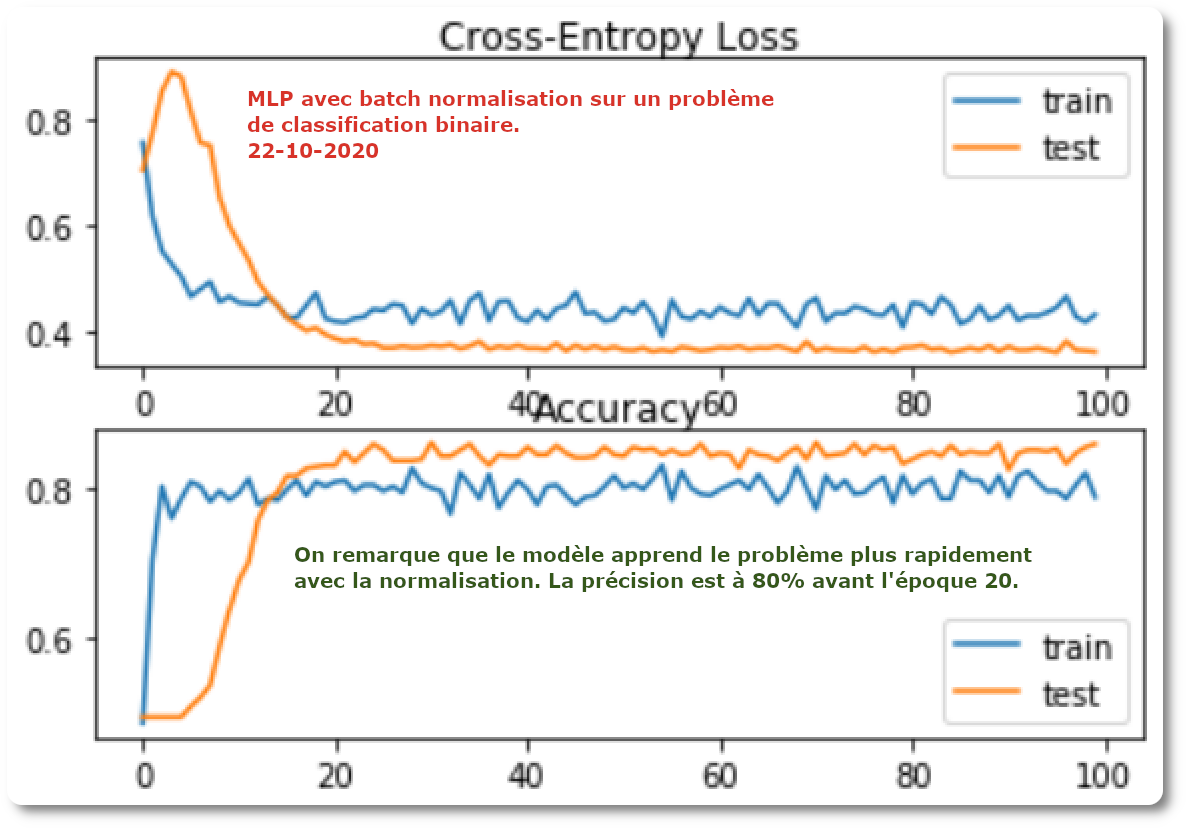
MLP on binary classification with batch normalization after activation function

MLP on binary classification with batch normalization after activation function

Chapter 10: Deeper models with greedy layer-wise pre-training

• As the number of hidden layers is increased, the amount of error information propagated back to earlier layers is dramatically reduced. This means that weights in hidden layers close to the output layer are updated normally, whereas weights in hidden layers close to the input layer are updated minimally or not at all. Generally, this problem prevented the training of very deep neural networks and was referred to as the vanishing gradient problem. An important milestone in the resurgence of neural networks that initially allowed the development of deeper neural network model was the technique of greedy layer-wise pre-training, often simply referred to as pre-training.
• Pre-training involves successively adding a new hidden layer to a model and refitting, allowing the newly added model to learn the inputs from the existing hidden layer, often while keeping the weights for the existing hidden layers fixed. This gives the technique the name layer-wise as the model is trained one layer at a time. The technique is referred as greedy because because of the piecewise or layer-wise approach to solving the harder problem of trains a deep network.
• "Greedy algorithms break a problem into many components, then solve for the optimal version of each component in isolation"..."builds on the premise that training a shallow network is easier than training a deep one."
• Although the weights in prior layers are held constant, it is common to fine tune all weights in the network at the end after the addition of the final layer.
• There are two main approaches to pre-training:
• supervised greedy layer-wise pre-training
• unsupervised greedy layer-wise pre-training: we can expect unsupervised pretraining to be most helpful when the number of labels is very small. Today, unsupervised pretraining has been largely abandoned, except in the field of natural language processing.

Case study

• Supervised greedy layer-wise pre-training:

Supervised greedy layer-wise pre-training model

• Unsupervised greedy layer-wise pre-training:
  
  Unsupervised greedy layer-wise pre-training
  
  
  
  

Chapter 11: Jump-start training with transfer learning

• An interesting benefit of deep learning neural networks is that they can be reused on related problems. Transfer learning refers to a technique for predictive modeling on a different but somehow similar problem that can be reused partly or wholly to accelerate the training and improve the performance of a model on the problem of interest.
• For example, we may learn about one set of visual categories, such as cats and dogs, in the first setting, then learn about a different set of visual categories, such as ants and wasps, in the second setting.
• Transfer learning has the benefit of decreasing the training time for a neural network model, resulting in lower generalization error.

Case study

• Step #1: A small multi class classification problem is used. A first problem will be trained and the weights of this model will be stored and used to for the second problem.

Problem 1 and 2 with three classes

• Step #2: We develop a MLP for problem #1 and save the model so that we can reuse the weights later:

Loss and accuracy learning curves on the train and test datasets for an MLP

• Step #3: We develop a MLP now for problem 2 that we will use as a baseline:

Loss and accuracy learning curves on the train and test datasets for an MLP

• Step #4: We are now using the weights of MLP problem #1 to fit the MLP problem #2

Loss and accuracy learning curves on the train and test sets for an MLP with transfer learning on problem #2

• Final step: We evaluate the transfer learning by performing 30 repeats to have an average performance. This together with a parameter which is the number of layers that we update or not with weights:
  
  Comparing standalone and transfer learning model
  
  

Conclusion

• By simply adding batch normalization before the activation function of a MLP neural network, the speed of learning is increased and needs twice as less epochs compared to a scenario without normalization.
• Pre-training may be useful for problems with small amounts labeled data and large amounts of unlabeled data.
• Transfer learning is a method for reusing a model trained on a related predictive modeling problem.
• Thanks to Jason Brownlee for the code and for his explanation.