europe: Better Deep Learning - Jason Brownlee (Chapter 5 and 6)

This post is the followup of the first part of the book "Deep Learning".
This post is a summary of the very best parts of the book "Deep Learning" from Jason Brownlee.
In this post, you will get information about:

How to configure the speed of learning with Learning rate
Stabilize learning with data scaling

Abondance, Alpes

Chapter 5: configure speed of learning with Learning Rate

The weights of a neural network cannot be calculated using an analytical method. Instead, the weights must be discovered via an empirical optimization procedure called stochastic gradient descent.
The amount of change to the model during each step of this search process, or the step size, is called the learning rate and provides perhaps the most important hyperparameter to tune for your neural network in order to achieve good performance on your problem.
Deep learning neural networks are trained using the stochastic gradient descent algorithm. Stochastic gradient descent is an optimization algorithm that estimates the error gradient for the current state of the model using examples from the training dataset, then updates the weight of the model using the back propagation of errors algorithm, referred to as simply as backpropagation.
The amount that the weights are updated during training is referred to as the step size or the learning rate. Specifically, the learning rate is a configurable hyperparameter used in the training of neural networks that has a small positive value, often in the range between 0.0 and 1.0.
The learning rate controls the amount of apportioned error that the weights of the model are updated with each time they are updated, such as at the end of each batch of training examples.
We should not use a learning rate that is too large or too small.
The learning rate may, in fact, be the most important hyperparameter to configure for your model.
Smaller batch sizes are better suited to smaller learning rates given the noisy estimate of the error gradient.
Diagnostic plots can be used to investigate how the learning rate impacts the rate of learning and learning dynamics of the model. One example is to create a line plot of loss over training epochs during training.

Case study on multi class classification problem

Different learning rates

Training a neural network can be made easier with the addition of history to the weight update. Specifically, an exponentially weighted average of the prior updates to the weight can be included when the weights are updated. This change to stochastic gradient descent is called momentum and adds inertia to the update procedure, causing many past updates in one direction to continue in that direction in the future.
The method of momentum is designed to accelerate learning.
Momentum is set to a value greater than 0.0 and less than one, where common values such as 0.9 and 0.99 are used in practice.

Suite of momentums

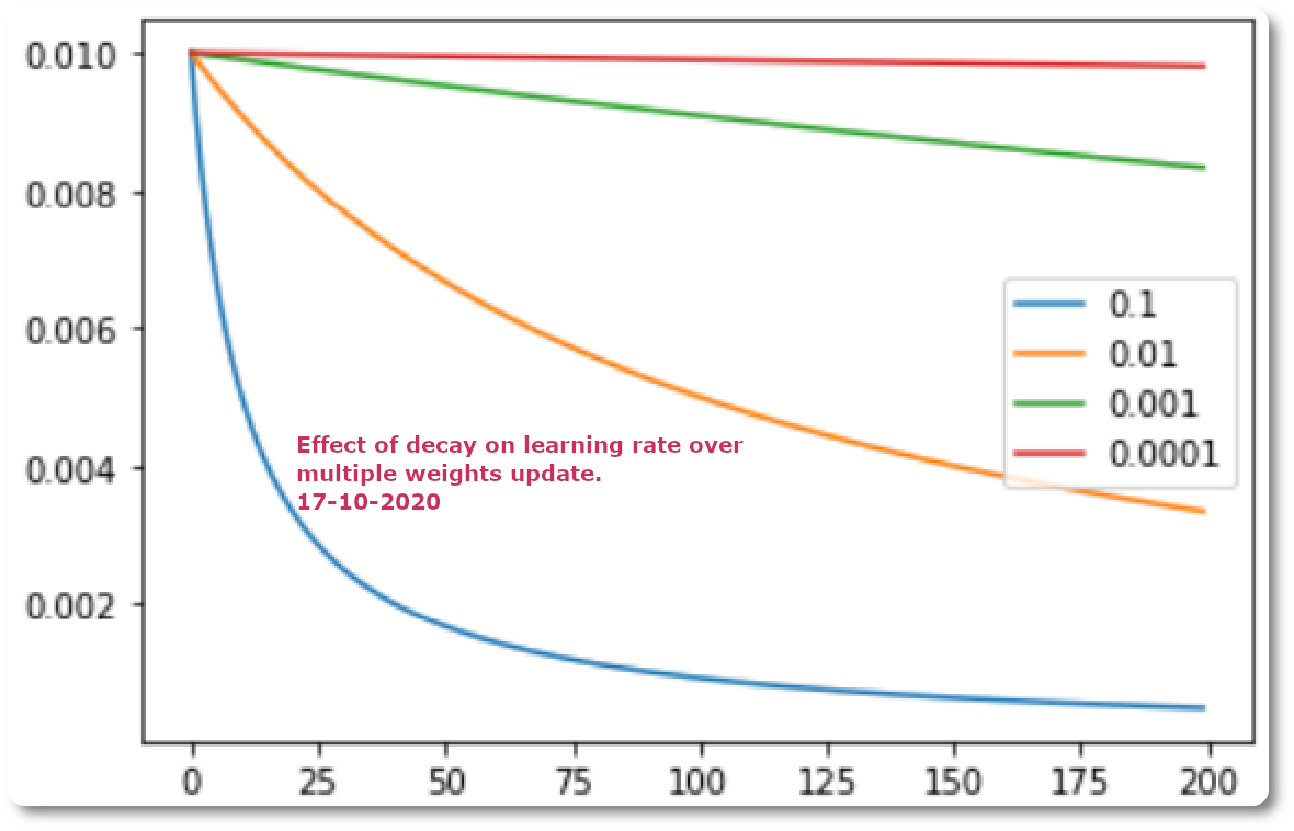
An alternative to using a fixed learning rate is to instead vary the learning rate over the training process. The way in which the learning rate changes over time (training epochs) is referred to as learning rate schedule or learning rate decay. Perhaps the simplest learning rate schedule is to decrease the learning rate linearly from a large initial value to a small value. This allows large weight changes in the beginning of the learning process and small changes or fine-tuning towards the end of the learning process.
Instead of choosing a fixed learning rate hyperparameter, the configuration challenge involves choosing the initial learning rate and a learning rate schedule.

Effect of decay on Learning Rate over multiple weight updates

Suite of decay rates

Adaptive learning rate: the performance of the model on the training dataset can be monitored by the learning algorithm and the learning rate can be adjusted in response.
There are three adaptive learning rate methods that have proven to be robust over many types of neural network architectures and problem types. They are AdaGrad, RMSProp, and Adam and all maintain and adapt the learning rates for each of the weights in the model. Perhaps the most popular is Adam, as it builds upon RMSProp and adds momentum.
Keras supports rate schedules via callbacks.
Keras provides the ReduceLROnPlateau callback that will adjust the learning rate when a plateau in model performance is detected, e.g. no change for a given number of training epochs.

Learning rate for different patience values used in the ReduceLROnPlateau schedule

Training loss over epochs for different patience values used in the ReduceLROnPlateau schedule

Accuracy over epochs for different patience values used in the ReduceLROnPlateau schedule

Accuracy for a suite of adaptive learning rate

Chapter 6: Stabilize Learning with Data Scaling

Given the use of small weights in the model and the use of error between predictions and actual values, the scale of inputs and outputs used to train the model are an in important factor. Unscaled input variables can result in a slow or unstable learning process, whereas unscaled target variables on regression problems can result in exploding gradients causing the learning process to fail. Data preparation involves using techniques such as normalization and standardization to rescale input and output variables prior to training a neural network model.
Differences in the scales across input variables may increase the difficulty of the problem being modeled.
Scaling input and output is a critical step in using neural network models.
A good rule of thumb is that input variables should be small values, probably in the range of 0-1 or standardized with a zero mean and a standard deviation of one.
If the distribution of the quantity is normal, then it should be standardized, otherwise the data should be normalized.
Normalization is a rescaling of the data from the original range so that all values are within the range of 0 and 1.
You can normalize your dataset using the scikit-learn object MinMaxScaler.
The default scale for the MinMaxScaler is to rescale variables into the range [0, 1], although a preferred scale can be specified via the feature_range argument and specify a tuple including the min and the max for all variables.
If needed, the transform can be inverted. This is useful for converting predictions back into their original scale for reporting or plotting. This can be done by calling the inverse_transform().
Standardizing a dataset involves rescaling the distribution of values so that the mean of observed values is 0 and the standard deviation is 1. It is sometimes referred to as whitening.
Standardization assumes that your observation fit a Gaussian distribution (bell curve) with a well behaved mean and standard deviation.
You can standardize your dataset using the scikit-learn object StandardScaler.

Data Scaling Case Study

A regression predictive problem involves predicting a real-value-quantity. We can use a standard regression problem generator provided by the scikit-learn library in the make_regression() function.

Histograms of two of the twenty input variables for the regression problem

Histogram de la variable cible pour le problème de régression

We run then a classical MLP model and the result is:

Example output from evaluating an MLP model on the unscaled regression problem

This demonstrates that, at the very least, some data scaling is required for the target variable. A line plot of training history is created but does not show anything as the model almost immediately results in a NaN mean squared error.