Preamble
- This is a followup of previous post about the excellent book from Jason Brownlee: "Generative Adversarial Networks with Python"
 Cercié en Beaujolais - Août 2020

Part III: GAN Evaluation
Chapter 11: How to Evaluate Generative Adversarial Networks
- Both the generator and discriminator are trained together to maintain an equilibrium.
- Models must be evaluated using the quality of the generated synthetic images.
- One training epoch refers to one cycle through the images in the training dataset used to update the model.
- Crowdsourcing platform like Amazon's Mechanical Turk.
- Two widely adopted metrics for evaluating generated images are the Inception Score and the Frechet Inception Distance. Like the inception score, the FID score uses the inception v3 model. The Frechet distance is also called the Wasserstein-2 distance. A lower FID score indicates more realistic images that match the statistical properties of real images.
- Once your confidence in developing GAN models improves, both the Inception Score and the Frechet Inception Distance can be used to qualitatively summarize the quality of generated images.
Chapter 12: How to Implement the Inception Score
- The Inception Score, or IS for short, is an objective metric for evaluating the quality of generated images, specifically synthetic images output by generative adversarial network models.
- The score seeks to capture two properties of a collection of generated images: image quality and image diversity.
Chapter 13: How to Implement the Frechet Inception Distance
- The Frechet Inception Distance, or FID for short, is a metric that calculates the distance between feature vectors calculated for real and generated images.
- The difference of two Gaussians (synthetic and real-world images) is measured by the Frechet distance also known as Wasserstein-2 distance.
Part IV: GAN Loss
Chapter 14: How to Use Different GAN Loss Functions
- The GAN architecture is relatively straightforward, although one aspect that remains challenging for beginners is the topic of GAN loss functions. The main reason is that the architecture involves the simultaneous training of two models: the generator and the discriminator. The discriminator model is updated like any other deep learning neural network, although the generator uses the discriminator as the loss function, meaning that the loss function for the generator is implicit and learned during training.
- The generative adversarial network, or GAN for short, is a deep learning architecture for training a generative model for image synthesis. They have proven very effective, achieving impressive results in generating photorealistic faces, scenes and more.
- The generator is not trained directly and instead is trained via the discriminator model. Specifically, the discriminator is learned to provide the loss function for the generator.
- The choice of a loss function is a hot research topic and many alternate loss functions have been proposed and evaluated. Two popular alternate loss functions used in many GAN implementations are the least squares loss and the Wasserstein loss.
- Despite a very rich research activity leading to numerous interesting GAN algorithms, it is still very hard to assess which algorithm(s) perform better than others.
Chapter 15: How to Develop a Least Squares GAN (LSGAN)
- The generator is updated in such a way that it is encouraged to generate images that are more likely to fool the discriminator. The discriminator is a binary classifier and is trained using binary cross-entropy loss function.
- The choice of cross-entropy loss means that points generated far from the boundary are right or wrong, but provide very little gradient information to the generator on how to generate better images. This small gradient for generated images far from the decision boundary is referred to as a vanishing gradient problem or a loss saturation. The loss function is unable to give a strong signal as to how to best update the model.
- The LSGAN is a modification to the GAN architecture that changes the loss function for the discriminator from binary cross-entropy to a least squares loss. The motivation for this change is that the least squares loss penalize generated images based on their distance from the decision boundary. This will provide a strong gradient signal for generated images that are very different or far from the existing data and address the problem of saturated loss.
- The LSGAN can be implemented by using the target values of 1.0 for real and 0.0 for fake images and optimizing the model using the mean squared error (MSE) loss function, e.g. L2 loss. The output layer of the discriminator model must be a linear active function.
- The generator model is updated via the discriminator model. This is achieved by creating a composite model that stacks the generator on top of the discriminator so that error signals can flow back through the discriminator to the generator. The weights of the discriminator are marked as not trainable when used in the composite model.
- The LSGAN addresses vanishing gradients and loss saturation of the deep convolutional GAN.
- The LSGAN can be implemented by a mean squared error or L2 loss function for the discriminator model.
- I ran the code provided by Jason on my Anaconda configuration and iMac Hardware. The code is an example of training on a MNIST dataset.The training lasted 3 hours and 26 minutes on my iMac.

100 LSGAN Generated Handwritten Digits after 1 training epoch

100 LSGAN Generated Handwritten Digits after 20 training epochs
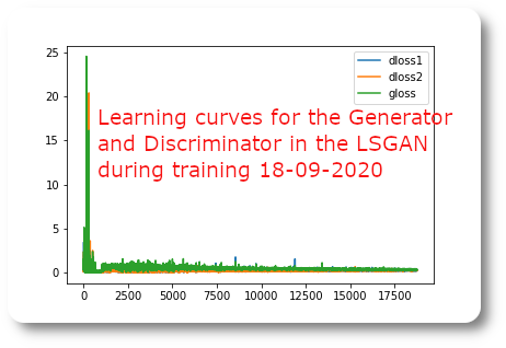
Learning curves for the Generator and Discriminator
- I ran the code to infer a new set of handwritten digits by using the trained model saved previously for 20 epochs:

100 LSGAN generated plausible handwritten digits
- Once the model has been trained, the inference is very fast to generate and the numbers are quite plausible.
Chapter 16: How to Develop a Wasserstein GAN (WGAN)
- The Wasserstein Generative Adversarial Network, or Wasserstein GAN, is an extension to the generative adversarial network that both improves the stability when training the model and provides a loss function that correlates with the quality of generated images. The development of the WGAN has a dense mathematical motivation, although in practice requires only a few minor modifications to the established deep convolutional generative adversarial network, or DCGAN.
- Instead of using a discriminator to classify or predict the probability of generated images as being real or fake, the WGAN changes or replaces the discriminator model with a critic that scores the realness or fakeness of a given image. This change is motivated by a mathematical argument that training the generator should seek a minimization of the distance between the distribution of the data observed in the training dataset and the distribution observed in generated examples. The argument contrasts different distribution distance measures, such as Kullback-Leibler (KL) divergence, Jensen-Shannon (JS) divergence, and the Earth-Mover (EM) distance, the latter also referred to as Wasserstein distance.
- The benefit of the WGAN is that the training process is more stable and less sensitive to model architecture and choice of hyper parameter configurations.
- The lower the loss of the critic when evaluating generated images, the higher the expected quality of generated images. This is important as unlike other GANs that seek stability in terms of finding an equilibrium between two models, the WGNA seeks convergence, lowering generator loss.
- The calculations are straightforward to interpret once we recall that stochastic gradient descent seeks to minimize loss.
- I ran the WGAN code provided in the book with the MNIST dataset, which consists at generating the number "7". The result I got was interesting, as we see that the network diverges around epoch #400 and then stabilizes again around epoch #800. The generated images are of better quality even after 194 batches compared to the images generated at batch # 776.

Loss and accuracy for a Wasserstein GAN (10 epochs)
- The images of the "7" generated at batch #194:
 The images generated at batch # 194


The images generated at batch # 776

The images generated at batch # 970
- I ran again the WGAN, this time the critics of the fake skyrockets after batch #600:

Loss and accuracy of a Wasserstein GAN (2nd trial, 10 epochs))
- So I decided to run with doubling the number of epochs:

Wasserstein GAN (3rd trial, 20 epochs)
- I had difficulty to interpret the learning curves with this WGAN. The only thing I am sure is the quality of the generated images: you can observe that at batch #776 the quality of the images are disastrous, whereas at batch # 970 they are quite better. The analysis from Jason Brownlee is the following: "WGAN is quite different from the typical GAN (DCGAN). The difference in loss means we cannot interpret learning curves easily - if at all. For myself, I don't even try and instead try to focus on the images generated by the model".
- I ran the code to infer a new set of handwritten digit "7" by using the trained model saved previously for 20 epochs:

Sample of Generated Images of a Handwritten Number 7 at Epoch 1940 from a Wasserstein GAN
Conclusion
- The part IV of the book, GAN loss, was the most interesting. I have experimented the stochastic nature of a GAN.
- I will jump hastily into the next part of the book, part V: conditional GANs.
- Great thanks to Jason Brownlee, thanks to him I have enjoyed so much getting a new knowledge and at the same time practicing and experimenting GANs.
1 commentaire:
Very impressive write-up!
Enregistrer un commentaire